In the Quantitative Trait Locus (QTL) analysis, composite interval mapping (CIM) method estimates the QTL positon with higher accuracy and statistical significance by combining interval mapping with multiple regression. This method also controls background noise resulting from genetic variations in other regions of the genome that affect the detection of the true QTL. In this post, my objective is to describe and walk you through all the basic steps one might need run the composite inteval mapping in R software. For further descriptive information on R/qtl, please read the paper by Karl Broman at this link: http://www.rqtl.org/
To get started
Step 1. Download and install R software and R studio
- Download and install the latest version of the R software from this link
- Download and install R studio from this link
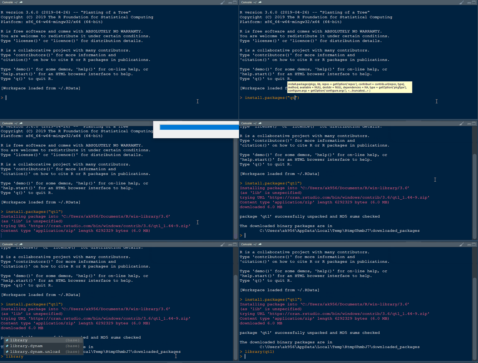
- Finally, install the library qtl in R
Step 1.1 - Install qtl library in R following the below steps:
Step 2. Prepare the input files
- Phenotype data
- Genetic map
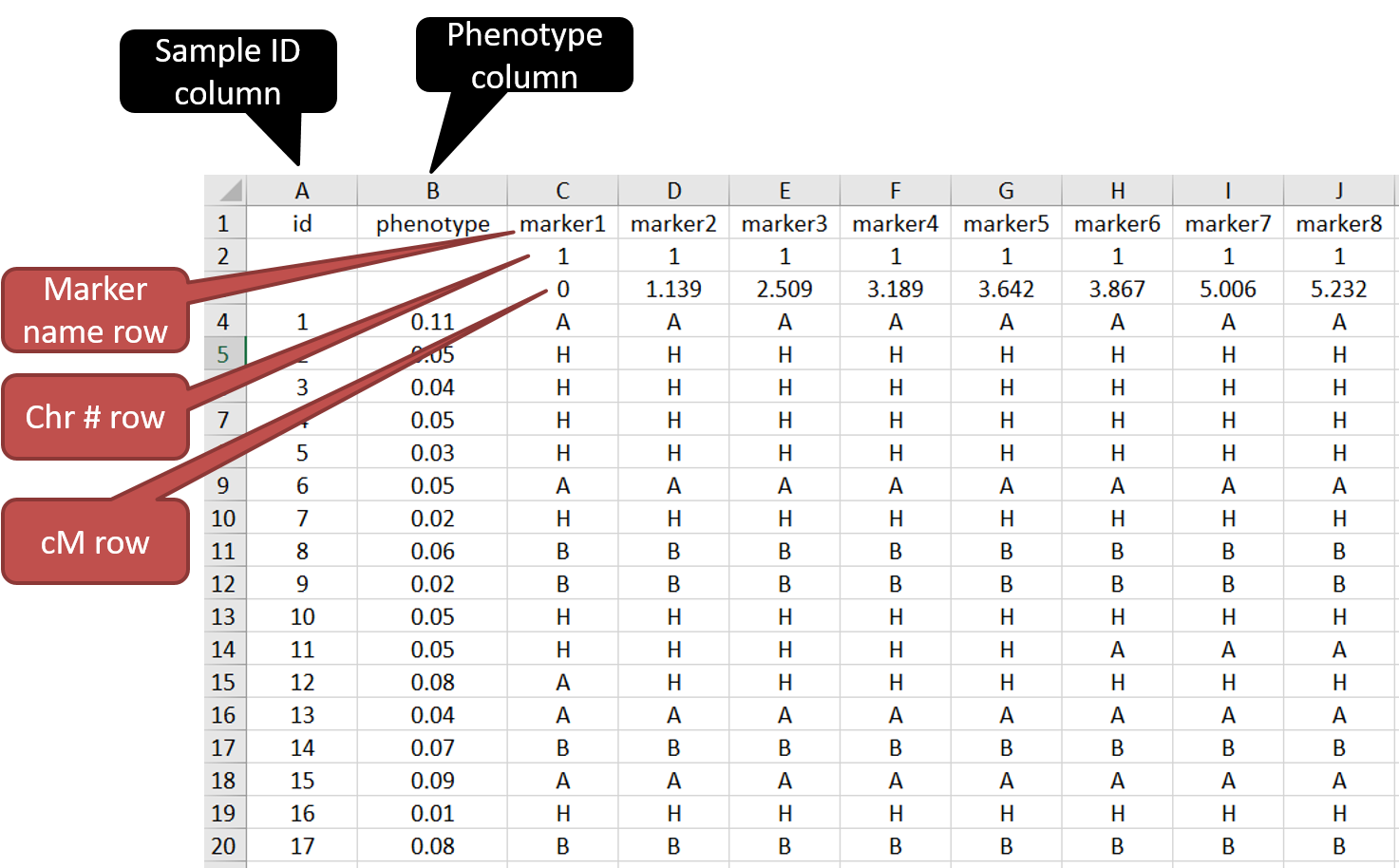
Both the phenotype and genetic map infomation can be put together in a single .csv file.
See below the screenshot to understand the formatting of the input file.
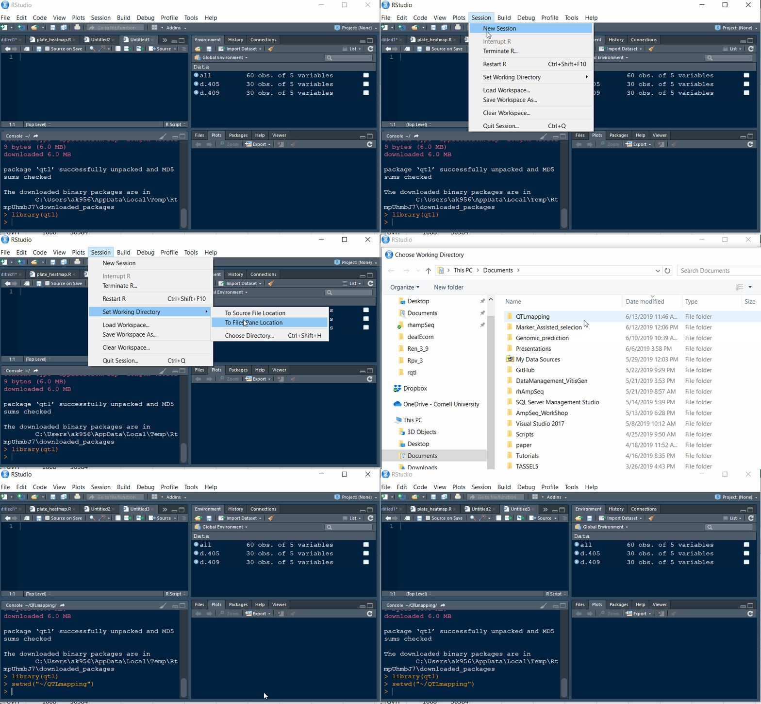
Step 2.1 - Setup working directory following the below steps:
Step 3. Running CIM in R
Please double check the formatting of the file is correct. Once ready, open R studio and type the following commands to get started.
Step 3.1. Import qtl library
library(qtl)
Step 3.2. Load the .csv file with the genotype and phenotype data
phenoGeno <-read.cross(format = "csv", file = "file.csv",
                 na.strings= c('NA'), genotypes = c("A","B","H"))
In the above command, if your genetic data is formatted differently then specify the in genotype section. To execute the above command, highlight the command and press CTRL + ENTER. You should see output in the terminal window, and please check for any warnings or errors.
Step 3.3. Summary of the data file and plotting
Type:
summary(phenoGeno)
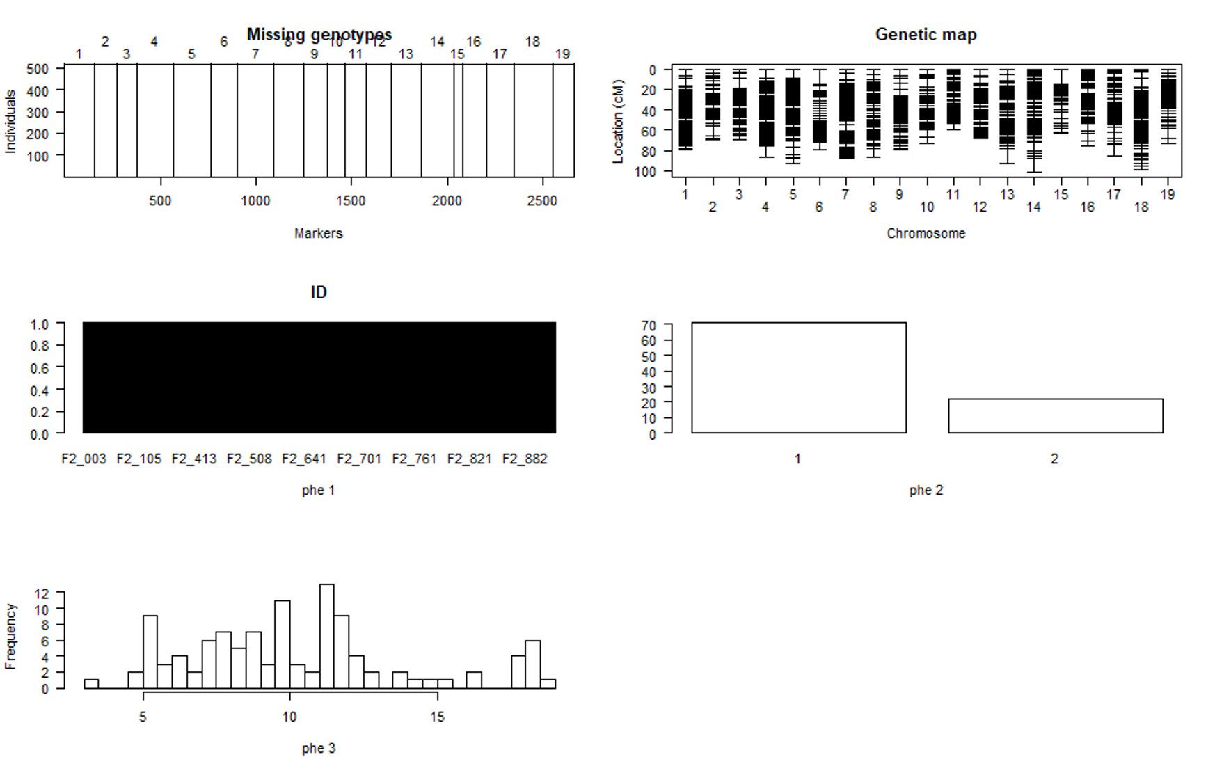
plot(phenoGeno)
You should see a plot similiar to shown below:
Step 3.4. Calculating genotype probabilities
In this step, Hidden Markov model technology is used to calculate the probabilities of the true underlying genotypes.
phenoGeno <- calc.genoprob(phenoGeno, step=0, off.end=0.0, error.prob=1.0e-4,stepwidth = "fixed", map.function="kosambi")

phenoGeno_cross <- sim.geno(phenoGeno,  n.draws=32, step=0, off.end=0.0, error.prob=1.0e-4, stepwidth = "fixed", map.function="kosambi")
Important Make sure to rename phenoGeno to phenoGeno_cross in the second step of the above command.
Step 3.5. running QTL scan using CIM method with permutations
- Type the below command in the console to run the qtl scan using
CIMmethod.scan.cim = cim(phenoGeno_cross, pheno.col=2, map.function="kosambi")Note In
#valuetype the column number of the phenotype - Run
permutationtest by typing the below command:scan.cim.perm = cim(phenoGeno_cross, pheno.col=2, map.function="kosambi", n.perm=1000)It is recommended to run at 1,000 permutation test.
- check the LOD threshold after permutations and significant QTL above the threshold.
summary(scan.cim.perm)
summary(scan.cim, threshold = #value)
Note In
#valueAdd the LOD score at desiredalpha(0.05 0r 0.1) - Plot the QTL scan
plot(scan.cim)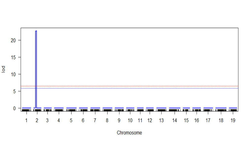
Step 4.0 QTL effect plot
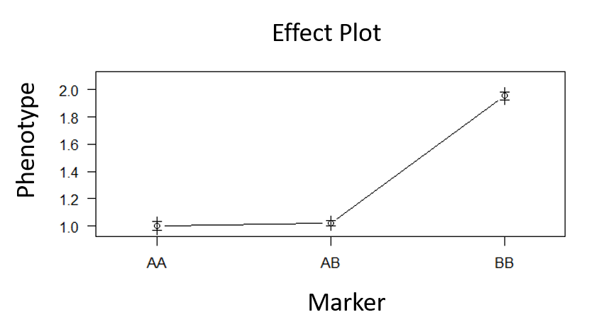
Type the below command to plot the effect plot of the QTL on the phenotype.
plotPXG(phenoGeno_cross, pheno.col = #value, marker = c("#value"))
Provide phenotype colum number in pheno.col and marker name in marker =
Output:
Step 5.0 Make QTL model with the significant marker
qtl <- makeqtl(phenoGeno_cross, chr=c(#value), pos=c(#value),what=c("prob"))

fitqtl <- fitqtl(don, pheno.col=c(#value), formula = y~Q1, qtl= qtl, method = "hk", get.ests = T)

summary(fitqtl)
Note In #value Add the signifincat marker’s coordinates i.e. chromosome and pos.
Below is the screenshot of the output one might except to see in the R shell:
fitqtl summary

Method: Haley-Knott regression
Model:  normal phenotype
Number of observations : 93

Full model result
----------------------------------
Model formula: y ~ Q1

      	df    SS   MS   LOD    %var 	Pvalue(Chi2) Pvalue(F)
Model 	 2  13.07	6.53  30.4  77.8           0         0
Error	 90  3.724093 0.04137881
Total	 92 16.795699

Estimated effects:
-----------------
               est       SE      t
Intercept  3.01835  0.09467 31.882
9@2.5a    -0.22761  0.09566 -2.379
9@2.5d    -1.41852  0.18935 -7.492
Note: Additive effect (a) = (BB - AA)/2 and Dominance effect (d) = AB - (AA + BB)/2.
Step 6.0 Identify QTL intervals using LOD drop
lodint(results = scan.cim, chr = #value, drop = 1.8)
Provide the cM to drop in the drop = and the chr
An example output is show below:
>   lodint(scan.cim, chr=2, drop=1.8)
           chr    pos      lod
2_14850509   3 45.290 11.44917
2_15846197   3 48.827 14.43254
2_19297395   3 50.312 12.45010
--- End of Tutorial ---
Thank you for reading this tutorial. I really hope this helpful in giving you the concept and technology behind AmpSeq and the data analysis. If you have any questions or comments, please let comment below or send me an email.
Bibliography
Broman KW, Wu H, Sen Ś, Churchill GA (2003) R/qtl: QTL mapping in experimental crosses. Bioinformatics 19:889-890 [PubMed | pdf (236k) | Screen pdf (288k)]