ANOVA also known as Analysis of Variance is a powerful statistical method to test a hypothesis involving more than two groups (also known as treatments). However, ANOVA is limited in providing a detailed insights between different treatments or groups, and this is where, Tukey (T) test also known as T-test comes in to play. In this tutorial, I will show how to prepare input files and run ANOVA and Tukey test in R software. For detailed information on ANOVA and R, please read this article at this link.

Step 1.0 Download and install R software and R studio

1. Download and install the latest version of the R software from this link
2. Download and install R studio from this link
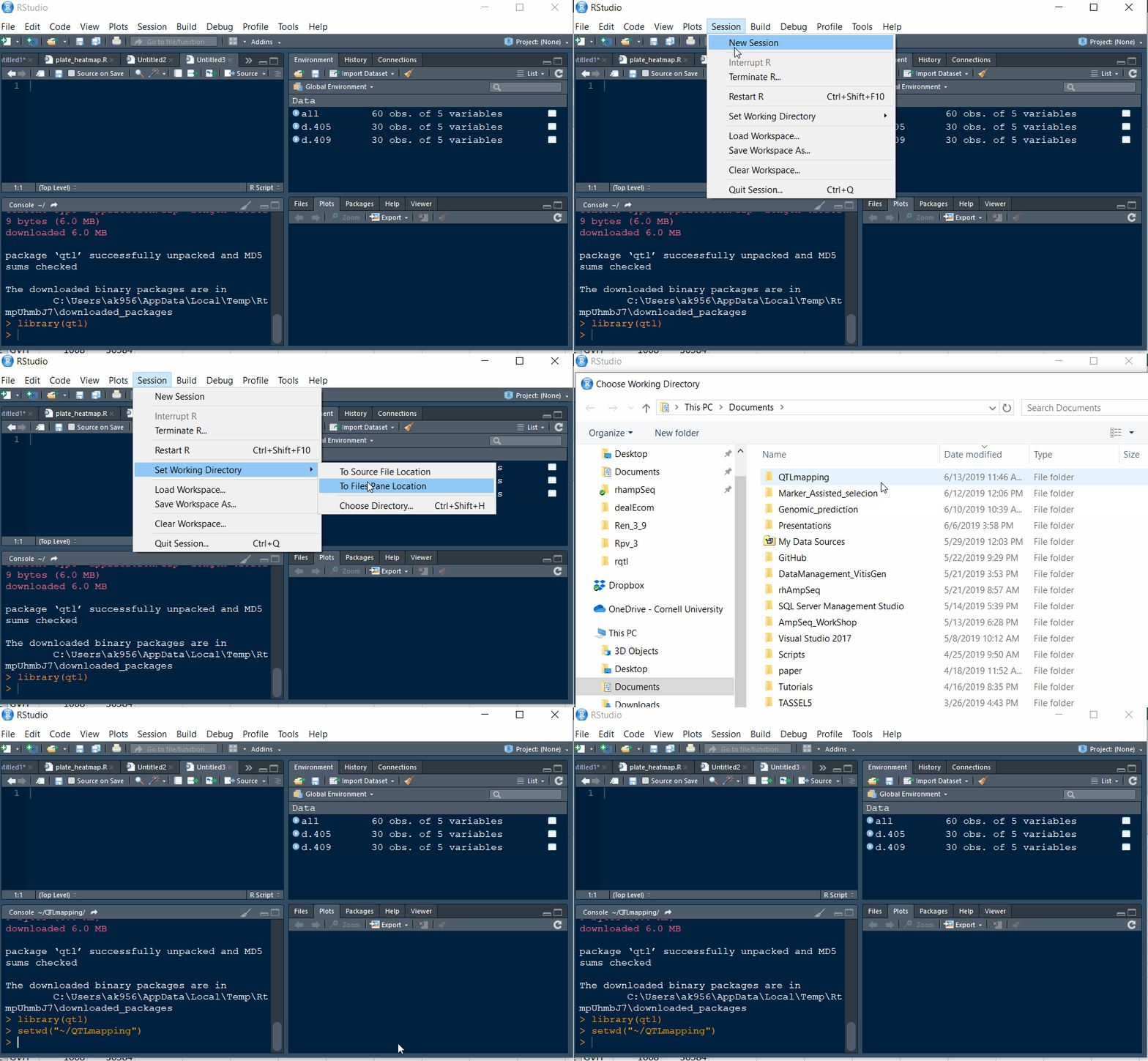
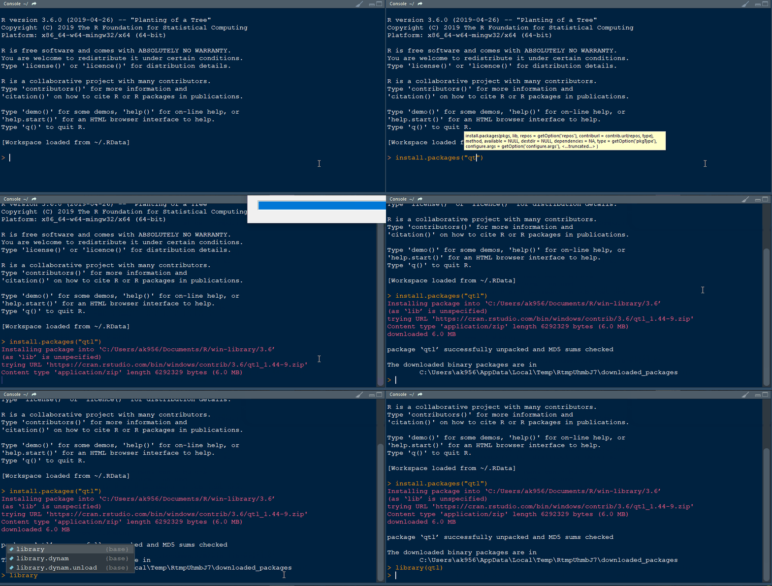
3. Finally, install the library qtl in R

Step 1.2 - Setup working directory following the below steps:

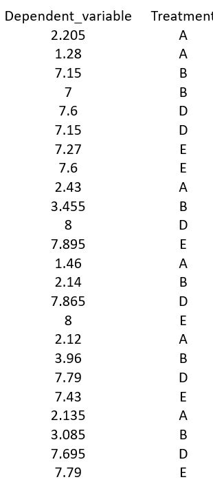
Step 1.3: Preparing the Input file

Create an input file as shown in the example below:

2.1 Import R package

Install R package agricolae and open the library typing the below command line:

library(agricolae)

Note: Please remember to install the correct R package for ANOVA!

2.2 Import data

Import your data by typing the below command line:

data= read.table(file = "fileName.txt", header = T)

2.3 Check data

Once the data is imported, check it by typing the below command line:

head(data_pressure)
tail(data_pressure)

2.4 Conduct ANOVA

Now, Simply run ANOVA by typing the below command lines:

data.lm <- lm(data$Dependent_variable ~ data$Treatment, data = data)

data.av <- aov(data.lm)
summary(data.av)

2.5 Regression Coefficient

Obtain regression coefficient of the predictors in the data using below code:

summary(data.lm)

Output –>

> summary(data.lm)

Call:
lm(formula = data$Dependent_variable ~ data$Treatment, data = data)

Residuals:
     Min       1Q   Median       3Q      Max 
-2.32500 -0.48500  0.05917  0.23979  2.68500 

Coefficients:
                Estimate Std. Error t value Pr(>|t|)    
(Intercept)       1.9383     0.4481   4.325 0.000329 ***
data$TreatmentB   2.5267     0.6338   3.987 0.000726 ***
data$TreatmentD   5.7450     0.6338   9.065 1.61e-08 ***
data$TreatmentE   5.7258     0.6338   9.035 1.70e-08 ***
---
Signif. codes:  0 ‘***’ 0.001 ‘**’ 0.01 ‘*’ 0.05 ‘.’ 0.1 ‘ ’ 1

Residual standard error: 1.098 on 20 degrees of freedom
Multiple R-squared:  0.8524,	Adjusted R-squared:  0.8302 
F-statistic: 38.49 on 3 and 20 DF,  p-value: 1.692e-08

To add another coefficient, add the symbol “+” for every additional variable you want to add to the model.

2.6 Overall model’s performance

The overall model’s performane cand be obtained using the below code:

summary(data.av)

Output –>

> summary(data.av)
               Df Sum Sq Mean Sq F value   Pr(>F)    
data$Treatment  3  139.2   46.38   38.49 1.69e-08 ***
Residuals      20   24.1    1.20                     
---
Signif. codes:  0 ‘***’ 0.001 ‘**’ 0.01 ‘*’ 0.05 ‘.’ 0.1 ‘ ’ 1

2.7 Good fit of the linear model

The coefficient of determination or R² is a good measure to test if the linear model has the good fit, and is measured by the proportion of the total variability explained by the regression model.

R² of a linear model can be obtained using below code:

summary(data.lm)$r.squared

Output –>

summary(data.lm)$r.squared
[1] 0.8523754

The model can explain ~85% of the total variability, which tells us that the model fits the data very well.

3.0 Conduct Tukey test

From the summary output, one can interpret that there is a significant difference (i.e. P < 0.001) between the Treatments, however, we perfom Tukey’s Test to investigate the differences between all treaments using steps below.

Type below commands to run Tukey test:

data.test <- TukeyHSD(data.av)
data.test

Below is the summary of the Tukey test:

> data.test
  Tukey multiple comparisons of means
    95% family-wise confidence level

Fit: aov(formula = data.lm)

$`data$Treatment`
           diff        lwr      upr     p adj
B-A  2.52666667  0.7527896 4.300544 0.0037260
D-A  5.74500000  3.9711229 7.518877 0.0000001
E-A  5.72583333  3.9519563 7.499710 0.0000001
D-B  3.21833333  1.4444563 4.992210 0.0003106
E-B  3.19916667  1.4252896 4.973044 0.0003326
E-D -0.01916667 -1.7930437 1.754710 0.9999897

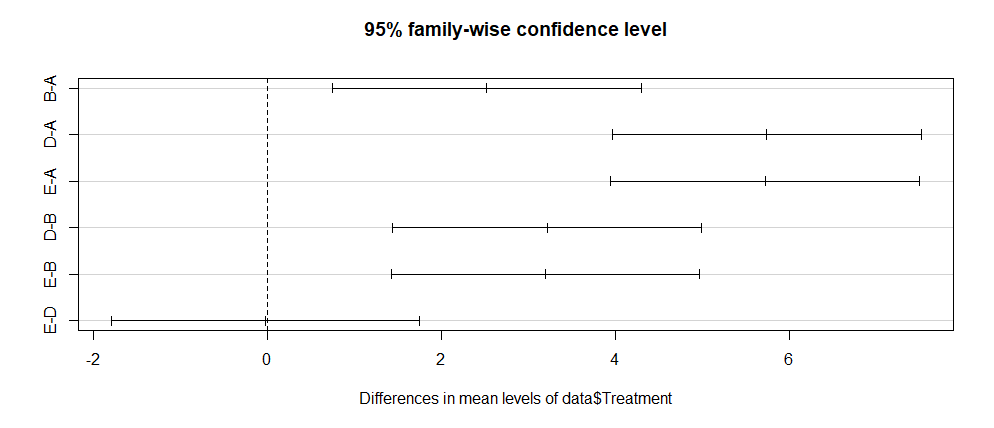
From the above T-test, one can conclude that there is a significant difference in the most of groups, except between-groups E-D at P <0.001

Finally, one can plot the above results using the below command:

plot(data.test)

Output:

Thank you for reading this tutorial. If you have any questions or comments, please let me know in the comment section below or send me an email.

Bibliography

Felipe de Mendiburu (2019). agricolae: Statistical Procedures for Agricultural Research. R package version 1.3-1. https://CRAN.R-project.org/package=agricolae