Multiple Quantitative traits were evaluated with varying heritabilties to study how the inheritance of a trait affect the performance of genomic selection and prediction models. Machine learning algorithms Random Forest and GLMnet: Lasso and Elastic-Net Regularized Generalized Linear Models were deployed to develop Genomic selection models using the publicly available dataset from the Maize genomes to fields (G2F) initiative. In the analysis, data from 40 maize hybrid experiments across 34 unique locations in 19 states in the U.S. and one Canadian province from years 2016 and 2017 experiments were evaluated.
From the data set, five important agronomic traits were selected: Days to Anthesis, Days to Silking, Plant height, Ear height and Grain yield, and exploratory data analysis of each trait by each year and across locations were explored as well as their heritability and BLUPs were calculated. Further, genotype-by-sequencing (GBS) for each hybrid in the dataset were filtered, thinned and imputed in command line TASSEL v5, prior to using them as predictors of the two quantitative traits. The two data sets: phenotype and genotype data were intersected by taxa and partioned into training and testing sets, and finally, training GS models were cross-validated on testing data set and evaluated by comparing the RMSE and R-Squared.
Table of Contents
- 1.0 Phenotypic data assessment
- 2.0 Genotypic data
- 3.0 Genomic selection algorithms
- 4.0 Summary of genomic selection algorithms on selected traits
1.0 Phenotypic data assessment
Download G2F phenotypic data from year 2016 and 2017
#install.packages("RCurl")
library(RCurl)

## download 2016 g2f hybrid clean (outliers removed) phenotypic data
download.file("https://de.cyverse.org/anon-files//iplant/home/shared/commons_repo/curated/GenomesToFields_2014_2017_v1/G2F_Planting_Season_2016_v2/a._2016_hybrid_phenotypic_data/g2f_2016_hybrid_data_clean.csv",destfile="pheno_2016_g2f_clean.csv",method="libcurl")

## download 2017 g2f hybrid clean (outliers removed) phenotypic data
download.file("https://de.cyverse.org/anon-files//iplant/home/shared/commons_repo/curated/GenomesToFields_2014_2017_v1/G2F_Planting_Season_2017_v1/a._2017_hybrid_phenotypic_data/g2f_2017_hybrid_data_clean.csv",destfile="pheno_2017_g2f_clean.csv",method="libcurl")
Import the downloaded two data sets in R environment
library(dplyr)

# import 2016 phenotype data
pheno_2016 <- read.csv(file = "pheno_2016_g2f_clean.csv", header = T, sep = ",",
                       na.strings = c("","NaN"), fileEncoding="UTF-8-BOM")


# import 2017 phenotype data
pheno_2017 <- read.csv(file = "pheno_2017_g2f_clean.csv", header = T, sep = ",",
                       na.strings = c("","NaN"), fileEncoding="UTF-8-BOM")
Checking the imported phenotype data
Code:
glimpse(pheno_2016)
View(pheno_2016)

glimpse(pheno_2017)
#View(pheno_2017)
Output:
 Rows: 16,377
 Columns: 38
 $ Year                                    <int> 2016, 2016, 2016, 2016, 201...
 $ Field.Location                          <chr> "ARH1", "ARH1", "ARH1", "AR...
 $ RecId                                   <int> 3094939, 3095402, 3093386, ...
 $ Source                                  <chr> "15SFG:2004", "15SJWE:G2F:1...
 $ Pedigree                                <chr> "2369/PHZ51", "LH195/PHN37"...
 $ Replicate                               <int> 2, 2, 2, 2, 1, 2, 1, 1, 2, ...
 $ Block                                   <int> 2, 2, 2, 2, 1, 2, 1, 1, 2, ...
 $ Plot                                    <int> 2, 53, 123, 137, 172, 217, ...
 $ Range                                   <int> 2, NA, 14, 15, 3, 17, 6, 3,...
 $ Pass                                    <int> 4, NA, 8, 7, 2, 7, 5, 9, 1,...
 $ LOCAL_CHECK..Yes..No.Blank..            <chr> NA, NA, NA, NA, NA, NA, NA,...
 $ Plot.Length.Field                       <dbl> 25, 25, 25, 25, 25, 25, 25,...
 $ Alley.Length                            <dbl> 5, 5, 5, 5, 5, 5, 3, 5, 5, ...
 $ Row.Spacing                             <int> 38, 38, 38, 38, 38, 38, 30,...
 $ Plot.Area                               <dbl> 126.67, 126.67, 126.67, 126...
 $ Rows.Plot                               <lgl> NA, NA, NA, NA, NA, NA, NA,...
 $ Packet.Plot                             <lgl> NA, NA, NA, NA, NA, NA, NA,...
 $ Kernels.Packet                          <lgl> NA, NA, NA, NA, NA, NA, NA,...
 $ X..Seed                                 <int> 98, 98, 98, 98, 98, 98, 100...
 $ Date.Planted                            <chr> "4/7/16", "4/7/16", "4/7/16...
 $ Date.Harvested                          <chr> "8/30/16", "8/30/16", "8/30...
Select five traits from the imported .csv data set from 2016 and 2017, and merging both data sets.
Code:
library(dplyr)
## 2016 selected phenotypes and creating new object
pheno_2016_selected <- pheno_2016 %>%
  dplyr::select(Pedigree, Year, Field.Location, Replicate, Block, Plot, Pollen.DAP..days., Silk.DAP..days., Plant.Height..cm., Ear.Height..cm., Grain.Yield..bu.A.)

head(pheno_2016_selected)


## 2017 selected phenotypes and creating new object
pheno_2017_selected <- pheno_2017 %>%
  dplyr::select(Pedigree, Year, Field.Location, Replicate, Block, Plot, Pollen.DAP..days., Silk.DAP..days., Plant.Height..cm., Ear.Height..cm., Grain.Yield..bu.A.)

head(pheno_2017_selected)

## merge selected 2016 and 2017 phenotype datya

merged_pheno <- rbind(pheno_2016_selected, pheno_2017_selected)
head(merged_pheno)
tail(merged_pheno)

#View(merged_pheno)
Output:
           Pedigree Year Field.Location Replicate Block Plot Pollen.DAP..days.
 1       2369/PHZ51 2016           ARH1         2     2    2                72
 2      LH195/PHN37 2016           ARH1         2     2   53                69
 3      PHHB9/PHM57 2016           ARH1         2     2  123                72
 4    PHW53/LH123HT 2016           ARH1         2     2  137                70
 5       B119/3IIH6 2016           ARH1         1     1  172                67
 6 BSSSC0_038/3IIH6 2016           ARH1         2     2  217                69
   Silk.DAP..days. Plant.Height..cm. Ear.Height..cm. Grain.Yield..bu.A.
 1              73               188             107          111.83608
 2              69               205             122          124.12257
 3              75               170             100           84.60683
 4              72               200              97          130.43523
 5              69               175             125          119.27595
 6              70               145              84           99.01134
Summary statistics table of the selected phenotpe data across years and locations
Code:
library(dplyr)
library(tidyr)

df_mergePheno <- tbl_df(merged_pheno)

df_mergePheno.summary <- df_mergePheno %>%
  dplyr::select(Pollen.DAP..days., Silk.DAP..days., Plant.Height..cm., Ear.Height..cm., Grain.Yield..bu.A.) %>% # select variables to summarise
  summarise_all(funs(min = min,
                      #q25 = quantile(., 0.25),
                      median = median,
                      #q75 = quantile(., 0.75),
                      max = max,
                      mean = mean,
                      sd = sd), na.rm = TRUE)

df_mergePheno.summary.tidy <- df_mergePheno.summary %>% gather(stat, val) %>%
  separate(stat, into = c("Phenotype", "stat"), sep = "_") %>%
  spread(stat, val) %>%
  dplyr::select(Phenotype, min, max, mean, median, sd ) # reorder columns

print(df_mergePheno.summary.tidy)
Output:
 # A tibble: 5 x 6
   Phenotype            min   max  mean median    sd
   <chr>              <dbl> <dbl> <dbl>  <dbl> <dbl>
 1 Ear.Height..cm.    20     266  106.    107  30.2
 2 Grain.Yield..bu.A.  7.97  323. 143.    145. 47.7
 3 Plant.Height..cm.  71     347  218.    225  49.2
 4 Pollen.DAP..days.  29      96   68.2    68   8.94
 5 Silk.DAP..days.    29      99   69.3    70   9.01
From the above table, Plant height and grain yield has the highest variance, while flowering time data has the lowest variance.
Data visualization
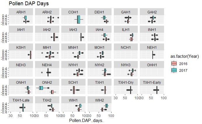
Box plots of each phenotype by year and multiple location.
Flowering time data
library(ggplot2)

## Pollen DAP days
ggplot(merged_pheno, aes(x=Pollen.DAP..days., fill = as.factor(Year))) +
geom_boxplot(alpha=0.6) + facet_wrap(~Field.Location) +
  scale_x_log10() +
  ggtitle("Pollen DAP Days")
Output:
## Silk.DAP..days.
ggplot(merged_pheno, aes(x=Silk.DAP..days., fill = as.factor(Year))) +
geom_boxplot(alpha=0.6)  + facet_wrap(~Field.Location) +
  scale_y_log10() +
  ggtitle("Silk DAP Days")
Output:
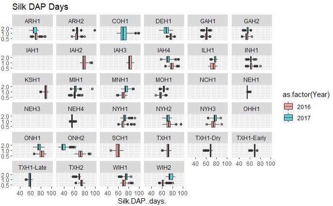
From the above plot, both flowering time data are consistent among two years and across years, however, with a couple of exceptions such as data from ONH2 (Canada), which appears to early flowering in 2017 and late in 2016, possibly due to difference in the weather conditions. Similarly, there are locations were no data were collected and or with only single year data.
Plant and ear height
# Plant height
ggplot(merged_pheno, aes(x=Plant.Height..cm., fill = as.factor(Year))) +
geom_boxplot(alpha=0.6)  + facet_wrap(~Field.Location) +
  scale_x_log10() +
  ggtitle("Plant height (cm)")


# Ear height
ggplot(merged_pheno, aes(x=Ear.Height..cm., fill = as.factor(Year))) +
geom_boxplot(alpha=0.6)  + facet_wrap(~Field.Location) +
  scale_x_log10() +
  ggtitle("Ear height (cm)")
Output:
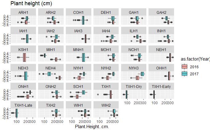
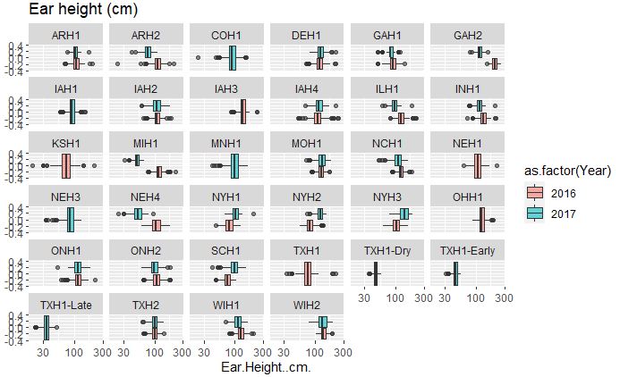
Both plant and ear height data across years and location are considerably consisent, with few outliers in the data set.
Grain Yield
# Grain Yield
ggplot(merged_pheno, aes(x=Grain.Yield..bu.A., fill = as.factor(Year))) +
geom_boxplot(alpha=0.6)  + facet_wrap(~Field.Location) +
  scale_x_log10() +
  ggtitle("Grain Yield (bu/Acre)")
Output:
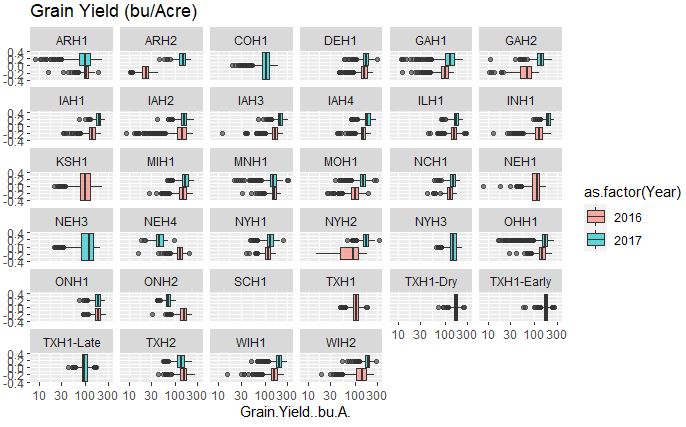
The grain yield that appears to fairly consistent between two years however, this data set has a high number of outliers in comparison to other traits.
Heritability
Calculating variance componets and Heritability on a line mean basis for each phenotype using lme4 package in R.
Checking data structure
attach(merged_pheno)

# checking data structure
str(merged_pheno)

# renaming variables

YEAR = as.factor(Year)
LINE = as.factor(Pedigree)
REP = as.factor(Replicate)
BLOCK = as.factor(Block)
LOC = as.factor(Field.Location)
POLLEN = as.numeric(Pollen.DAP..days.)
SILK = as.numeric(Silk.DAP..days.)
EAR_HT = as.numeric(Ear.Height..cm.)
PLNT_HT = as.numeric(Plant.Height..cm.)
GRAIN_YLD = as.numeric(Grain.Yield..bu.A.)
output:
 'data.frame':    34758 obs. of  11 variables:
  $ Pedigree          : chr  "2369/PHZ51" "LH195/PHN37" "PHHB9/PHM57" "PHW53/LH123HT" ...
  $ Year              : int  2016 2016 2016 2016 2016 2016 2016 2016 2016 2016 ...
  $ Field.Location    : chr  "ARH1" "ARH1" "ARH1" "ARH1" ...
  $ Replicate         : int  2 2 2 2 1 2 1 1 2 2 ...
  $ Block             : int  2 2 2 2 1 2 1 1 2 2 ...
  $ Plot              : int  2 53 123 137 172 217 104 179 170 174 ...
  $ Pollen.DAP..days. : int  72 69 72 70 67 69 62 67 67 67 ...
  $ Silk.DAP..days.   : int  73 69 75 72 69 70 63 69 69 69 ...
  $ Plant.Height..cm. : num  188 205 170 200 175 145 244 183 177 146 ...
  $ Ear.Height..cm.   : num  107 122 100 97 125 84 124 114 109 96 ...
  $ Grain.Yield..bu.A.: num  111.8 124.1 84.6 130.4 119.3 ...
Pollen DAP data
library(lme4)

## Model variance component analysis

pollen_varcomp = lmer(POLLEN ~ (1|LINE) + (1|LOC) + (1|YEAR) +  (1|LINE:LOC) + (1|LINE:YEAR))

summary(pollen_varcomp)

## formula calucalting heritability on mean basis
# H2 = var(LINE)/[var(LINE) + var(LINE:LOC)/N] + var(LINE:YEAR)/N + var(RESIDUAL)/N]

H2_pollen = 10.47035 /(10.47035 + 0.05196/34 + 0.13156/2 + 20.16058/36)

cat("Heritabilty of Pollen DAP days is", H2_pollen, "\n")
 Linear mixed model fit by REML ['lmerMod']
 Formula: POLLEN ~ (1 | LINE) + (1 | LOC) + (1 | YEAR) + (1 | LINE:LOC) +
     (1 | LINE:YEAR)

 REML criterion at convergence: 151506.8

 Scaled residuals:
     Min      1Q  Median      3Q     Max
 -5.1637 -0.4649  0.0036  0.4833  7.4742

 Random effects:
  Groups    Name        Variance Std.Dev.
  LINE:LOC  (Intercept)  0.05186 0.2277
  LINE:YEAR (Intercept)  0.13160 0.3628
  LINE      (Intercept) 10.47045 3.2358
  LOC       (Intercept) 78.26891 8.8470
  YEAR      (Intercept)  0.02846 0.1687
  Residual              20.16066 4.4901
 Number of obs: 25515, groups:
 LINE:LOC, 9242; LINE:YEAR, 1305; LINE, 815; LOC, 30; YEAR, 2

 Fixed effects:
             Estimate Std. Error t value
 (Intercept)   67.377      1.624   41.48
Silk DAP data
silk_varcomp = lmer(SILK ~ (1|LINE) + (1|LOC) + (1|YEAR) +  (1|LINE:LOC) + (1|LINE:YEAR))

summary(silk_varcomp)


# formula calucalting heritability on mean basis
# H2 = var(LINE)/[var(LINE) + var(LINE:LOC)/N] + var(LINE:YEAR)/N + var(RESIDUAL)/N]

H2_silk = 12.2271 /(12.2271 + 0.0155/34 + 0.2316/2 + 20.7834/36)

cat("Heritabilty of Silk DAP days is", H2_silk, "\n")
Plant height data
plantHT_varcomp = lmer(PLNT_HT ~ (1|LINE) + (1|LOC) + (1|YEAR) + (1|LINE:LOC) + (1|LINE:YEAR))

summary(plantHT_varcomp)

# formula calucalting heritability on mean basis
# H2 = var(LINE)/[var(LINE) + var(LINE:LOC)/N] + var(LINE:YEAR)/N + var(RESIDUAL)/N]

H2_plHT = 287.302 /(287.302 + 2.628/34 + 2.589/2 + 604.888/36)

cat("Heritabilty of ear height data is", H2_plHT, "\n")
Ear height data
earHT_varcomp = lmer(EAR_HT ~ (1|LINE) + (1|LOC) + (1|YEAR) + (1|LINE:LOC) + (1|LINE:YEAR))

summary(earHT_varcomp)

## formula calucalting heritability on mean basis
# H2 = var(LINE)/[var(LINE) + var(LINE:LOC)/N] + var(LINE:YEAR)/N + var(RESIDUAL)/N]

H2_earHT = 166.764 /(166.764 + 4.028/34 + 2.589/2 + 257.965/36)

cat("Heritabilty of ear height data is", H2_earHT, "\n")
Grain yield data
Yield_varcomp = lmer(GRAIN_YLD ~ (1|LINE) + (1|LOC) + (1|YEAR) + (1|LINE:LOC) + (1|LINE:YEAR))

summary(Yield_varcomp)

# formula calucalting heritability on mean basis
# H2 = var(LINE)/[var(LINE) + var(LINE:LOC)/N] + var(LINE:YEAR)/N + var(RESIDUAL)/N]

H2_yield = 187.64 /(187.64 + (92.85/34) + (54.95/2) + (1000.21/36))

cat("Heritabilty of ear height data is", H2_yield, "\n")
Summary table of the heritablity of each trait
| Trait | H2 |
|---|---|
| Pollen DAP | 0.94 |
| Silk DAP | 0.95 |
| Plant height | 0.94 |
| Ear height | 0.95 |
| Grain yield | 0.76 |
All traits have high broad-sense heritabilty except grain yield, which implies that the grain yield is significantly influenced by environmental and other unknown factors, and using only genetic markers for GS could result spurious results.
Estimating Best Linear UnBiased Predictors (BLUP) for each Line by trait
BLUPs shrink the estimates toward the mean and allow us to account for environmental, year-to-year variance factors in the model as well as the missing data.
Pollen DAP days
# estimate BLUPS
pollen_blup = ranef(pollen_varcomp)
# look at output structure
str(pollen_blup)
# extract blup for line
pollen_lineblup = pollen_blup$LINE
# see the structure of the blup for each line
str(pollen_lineblup)
# save the brixlineblup output to a separate .csv file
write.csv(pollen_lineblup, file="Pollen_LineBLUPS.csv")


LINEBLUP_pollen = pollen_lineblup[,1]
Silk DAP days
# estimate BLUPS
silk_blup = ranef(silk_varcomp)
# look at output structure
str(silk_blup)
# extract blup for line
silk_lineblup = silk_blup$LINE
# see the structure of the blup for each line
str(silk_lineblup)
# save the brixlineblup output to a separate .csv file
write.csv(silk_lineblup, file="silkDAP_LineBLUPS.csv")

LINEBLUP_silk = silk_lineblup[,1]
Plant height
# estimate BLUPS
plntHT_blup = ranef(plantHT_varcomp)
# look at output structure
str(plntHT_blup)
# extract blup for line
plntHT_lineblup = plntHT_blup$LINE
# see the structure of the blup for each line
str(plntHT_lineblup)
# save the brixlineblup output to a separate .csv file
write.csv(plntHT_lineblup, file="plntHT_LineBLUPS.csv")

LINEBLUP_plntHT = plntHT_lineblup[,1]
Ear height
# estimate BLUPS
earHT_blup = ranef(earHT_varcomp)
# look at output structure
str(earHT_blup)
# extract blup for line
earHT_lineblup = earHT_blup$LINE
# see the structure of the blup for each line
str(earHT_lineblup)
# save the brixlineblup output to a separate .csv file
write.csv(earHT_lineblup, file="earHT_LineBLUPS.csv")


LINEBLUP_earHT = earHT_lineblup[,1]
Grain Yield
# estimate BLUPS
yield_blup = ranef(Yield_varcomp)
# look at output structure
str(yield_blup)
# extract blup for line
yield_lineblup = yield_blup$LINE
# see the structure of the blup for each line
str(yield_lineblup)
# save the brixlineblup output to a separate .csv file
write.csv(yield_lineblup, file="yield_lineblup.csv")

LINEBLUP_yield = yield_lineblup[,1]
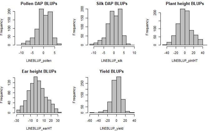
Histograms of the BLUPs for each trait
par(mfrow=c(2,3))
hist(LINEBLUP_pollen, col="grey", main = "Pollen DAP BLUPs")
hist(LINEBLUP_silk, col="grey", main = "Silk DAP BLUPs")
hist(LINEBLUP_plntHT, col="grey" , main = "Plant height BLUPs")
hist(LINEBLUP_earHT, col="grey", main = "Ear height BLUPs")
hist(LINEBLUP_yield, col="grey", main = "Yield BLUPs")
par(mfrow=c(1,1))
2.0 Genotypic data
The imputed genotpe data was downloaded from G2F_Planting_Season_2017_v1, with filename: g2f_2017_ZeaGBSv27_Imputed_AGPv4.h5 and analyzed on Cornell University BioHPC Cluster in Linux OS using command line version of TASSEL v5.
The genotype summary of the raw genetic data set was calculated in TASSEL command line.
Plot Minor and Major Allele Frequency raw marker data:
rawMarkerSum <- read.table("raw_geno_summary3.txt", header = T)

df_rawMF <- data.frame(MinorAlleleF=rawMarkerSum$Minor_Allele_Frequency,
                MajorAlleleF=rawMarkerSum$Major_Allele_Frequency)
library(ggplot2);library(reshape2)
rawdata<- melt(df_rawMF)
ggplot(rawdata, aes(x=value, fill=variable)) + geom_histogram(bins = 100) + ggtitle("Raw genotype allele freq.")
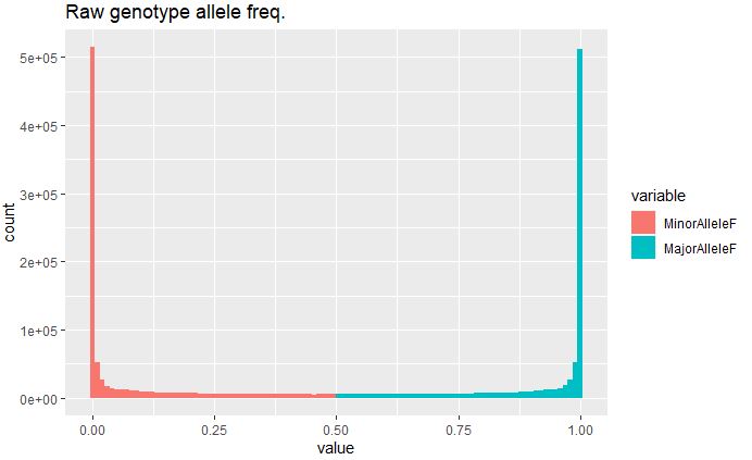
Minor allele frequency in the raw data is extremely high (<5e+05), indicating presence of rare variants in disproportionate number, and therefore needs to be filtered prior to any downstream analysis to avoid any bias in the result.
Filtering genotype calls of MAF and minimum site count
In TASSEL, SNP calls were filtered stringently for MAF threshold of 0.1 and minimum count of 1000 to remove extremely rare variants and the number of markers with high missing data. Similarly, taxa with greater 80% missing genotype calls were also filtered using the command line below.
$ ./tassel-5-standalone/run_pipeline.pl -log log.txt -Xms2g -Xmx10g  -fork1 -h5 genotype_imputed_2017.h5 -filterAlign -filterAlignMinFreq--exit-with-session 0.05 -filterAlignMinCount 200 -FilterTaxaPropertiesPlugin -minNotMissing 0.2 -endPlugin  -export -w
genotype_imputed_2017_filtered -exportType VCF -runfork1
Next, genotype summary of the filtered file was generated in TASSEL using -GenotypeSummaryPlugin and using the below command line:
$ ./tassel-5-standalone/run_pipeline.pl -Xmx20g -importGuess genotype_imputed_2017_filteredMAF01min1000.vcf -GenotypeSummaryPlugin -endPlugin -export GenoSummary_filtered
Summary of the 2017 genotypic data after filteration of markers and taxa
| Stat Type | Value |
|---|---|
| Number of Taxa | 1512 |
| Number of Sites | 232681 |
| Sites x Taxa | 3.5181E8 |
| Number Not Missing | 3.1629E8 |
| Proportion Not Missing | 0.89901 |
| Number Missing | 3.5528E7 |
| Proportion Missing | 0.10099 |
| Number Gametes | 7.0363E8 |
| Gametes Not Missing | 6.3257E8 |
| Proportion Gametes Not Missing | 0.89901 |
| Gametes Missing | 7.1057E7 |
| Proportion Gametes Missing | 0.10099 |
| Number Heterozygous | 8.114E6 |
| Proportion Heterozygous | 0.02306 |
| Average Minor Allele Frequency | 0.28261 |
Even after stringent filtering, there are about 10% missing data in filtered data set. But before that, the number of filtered markers or predictors are on higher end which could possibly be in high linkage disequilibrium (LD) with one another and not providing any additional importance in the analysis but adding computational burdern. Therefore, this marker set was further thinned by its physical position and imputed.
Thinning of markers by position
232,681 markers were obtained after post-filtering the raw marker set. To reduce the computational workload and redundant markers in strong LD, filtered marker set were thinned by their physical position using _ThinSitesByPositionPlugin with minimum physical distance between markers of 10,000 bp.
$ ./tassel-5-standalone/run_pipeline.pl -log log_thinMarkers.txt -Xmx20g -importGuess genotype_imputed_2017_filteredMAF01min1000.vcf -ThinSitesByPositionPlugin -o thinned10k_geno_2017.vcf -minDist 10000 -endPlugin
Summary of the markers after thinning them:
| Stat Type | Value |
|---|---|
| Number of Taxa | 1512 |
| Number of Sites | 28595 |
| Sites x Taxa | 4.3236E7 |
| Number Not Missing | 3.8758E7 |
| Proportion Not Missing | 0.89643 |
| Number Missing | 4.4779E6 |
| Proportion Missing | 0.10357 |
| Number Gametes | 8.6471E7 |
| Gametes Not Missing | 7.7515E7 |
| Proportion Gametes Not Missing | 0.89643 |
| Gametes Missing | 8.9558E6 |
| Proportion Gametes Missing | 0.10357 |
| Number Heterozygous | 1.0066E6 |
| Proportion Heterozygous | 0.02328 |
| Average Minor Allele Frequency | 0.27872 |
Proportion of missing genotype calls is same after thinning.
Plot MAF of thinned marker set:
thinSiteSum <- read.table("thinnedGeno_summary3.txt", header = T)

x <- data.frame(MinorAlleleF=thinSiteSum$Minor_Allele_Frequency,
                MajorAlleleF=thinSiteSum$Major_Allele_Frequency)
library(ggplot2);library(reshape2)
data<- melt(x)
ggplot(data,aes(x=value, fill=variable)) + geom_histogram(alpha=0.5, bins = 100) + ggtitle("Thinned genotype allele freq.")
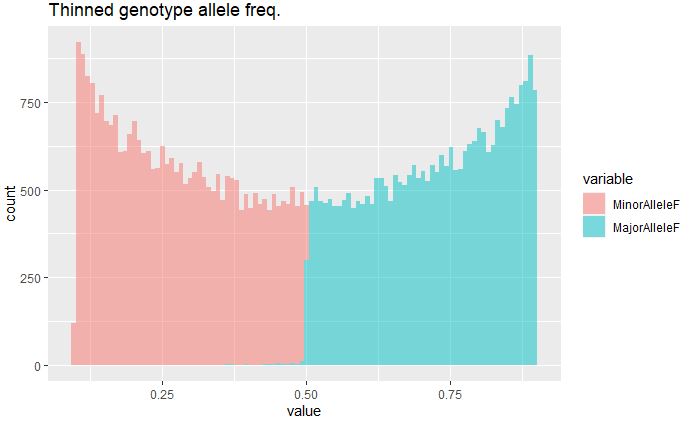
MAF post-filtering and thinning has removed most of the rare variants in the data set.
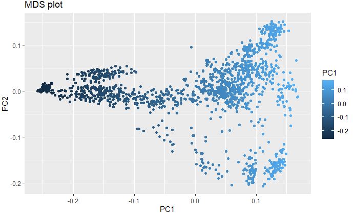
Plot Multidimenisonal Scaling (MDS) to explore genetic structure of the genotypes
MDS with elucidean distance was calcuated using post-filtered and thinned marker data to detect the underlying dimensions of the observed genetic distance i.e Identity-By-Descent (IBS) among the lines in the data set.
mds <- read.table("MDS_thinned10k_geno.txt", header = T)
head(mds)
ggplot(mds, aes(x=PC1, y=PC2, color = PC1))+
  geom_point() +
  ggtitle("MDS plot")
Converting thinned genotype data into numerical format and imputing for Machine Learning
28,595 markers post-filteration were converetd into numeric format using -NumericalGenotypePlugin in TASSEL (see log_numeric.txt file for details), where, for each marker homozygous major is 1.0, homozygous minor is 0.0, and heterozygous is 0.5 that will be used as predictors in the genomic selection analysis.
command line:
$ ./tassel-5-standalone/run_pipeline.pl -Xmx20g -log 10g_numeric.txt -importGuess thinned10k_geno_2017.vcf -NumericalGenotypePlugin -endPlugin -export Numeric_thinned_2017_geno -exportType ReferenceProbability
Running Numerical Imputation by means from TASSEL command line:
The numeric imputation was performed by computing the mean of the respective marker columns.
$ ./tassel-5-standalone/run_pipeline.pl -Xms10g -Xmx30g -log log_numericImpute.txt -importGuess Numeric_thinned_2017_geno.txt -ImputationPlugin -ByMean -endPlugin -export Numeric_thinned_2017_geno_Imputed -exportType ReferenceProbability
Intersecting genotype and phenotype data
pheno_BlUPs_noMissing <- read.table("pheno_BLUPs_allTraits_wGBStaxaNames_noMissingData.txt", header = T, na.strings = "NA")
geno_numericThinImpu <- read.table("Numeric_thinned_2017_geno_Imputed.txt", header = T)

## as data frames
pheno_BlUPs_noMissing <- as.data.frame(pheno_BlUPs_noMissing)
geno_numericThinImpu <- as.data.frame(geno_numericThinImpu)

head(pheno_BlUPs_noMissing)
#head(geno_numericThinImpu)
The phenotype and numerical genotype data were intersected by the Taxa names in each data set, and any Taxa with missing data were removed from the GS analysis.
## return all rows from x where there are matching values in y, and all columns from x and y
intrsct_phenoGeno <- inner_join(pheno_BlUPs_noMissing, geno_numericThinImpu)

head(intrsct_phenoGeno)
Output:
##                 Taxa  earBLUPs PlantHTBLUPs yield_BLUPs PollenDAP_BLUPs
## 1 PI601318:250033667 -29.39624    -23.67643    1.503655      -5.0852823
## 2 PI601170:250032540 -27.66371    -37.79167    1.988569      -5.2087454
## 3    PHJ89:100000663 -26.73055    -17.46497    6.775845      -5.4622321
## 4    S8324:100000684 -26.71990    -30.55353  -23.851084      -9.3000384
## 5     CG60:100001134 -26.41626    -40.89895  -16.331693      -6.9434702
## 6 PI601575:250035073 -26.06640    -31.77753    8.341925      -0.3779614
##   silkDAP_BLUPs
## 1    -5.1033176
## 2    -5.3709531
## 3    -5.5588561
## 4    -9.2906753
## 5    -7.8424272
## 6    -0.2195389
3.0 Genomic selection algorithms
In the GS analysis, BLUPs only two traits – Pollen DAP (high H2) and Grain yield (low H2) were evaluated, to evaluated the performance of GS alogrithms (Random Forest and Glmnet) on traits with significantly different heritability.
libraries and set seed
library(randomForest)
library(mlbench)
library(caret)
library(e1071)

set.seed(07232020)
Randomizing and Partitioning the dataset to build training and testing sets
The imported data was split into 70/30 split, since this dataset gives a larger and more reliable test set.
Randomizing the order of the dataset
rows <- sample(nrow(intrsct_phenoGeno))

intrsct_phenoGeno <- intrsct_phenoGeno[rows, ]
Find the rows to split
split <- round(nrow(intrsct_phenoGeno) * 0.70)

train_set <- intrsct_phenoGeno[1:split,]

test_set <- intrsct_phenoGeno[(split + 1):nrow(intrsct_phenoGeno),]
Confirm train and test set sizes
# Check the ratios of training and test sets
nrow(train_set)/nrow(intrsct_phenoGeno)

nrow(test_set)/nrow(intrsct_phenoGeno)

# plot the two data sets
par(mfrow=c(2,2))
hist(train_set$PollenDAP_BLUPs, main = "Train set - Pollen DAP", xlab = "Pollen DAP BLUPs")
hist(test_set$PollenDAP_BLUPs, main = "Test set - Pollen DAP", xlab = "Pollen DAP BLUPs")
hist(train_set$yield_BLUPs, main = "Train set - Grain Yield", xlab = "Grain Yield BLUPs")
hist(test_set$yield_BLUPs, main = "Test set - Grain Yield", xlab = "Grain Yield BLUPs")
par(mfrow=c(1,1))
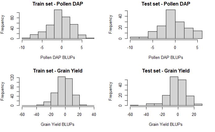
As needed, the distribution of training and testing set is about the same, which is import to prevent any bias in the result.
Pollen DAP BLUPs
glmnet model
It is a extension of glm models with a built-in variable selection that also help in dealing with collinearity and small sizes. The glmnet has two primary froms: 1) LASSO regression, which penalizes number of non-zero coefficients, and 2) Ridge regression, which penalizes absolute magnitude of coefficients. It also attempts to find a parsimonious aka simple model and pairs well with random forest models.
trainControl
Before creating and running the models, its a good idea to create a trainControl object to tuning parameters and further control how models are created.
myControl <- trainControl(
  method = "cv",
  number =10,
  summaryFunction = twoClassSummary,
  classProbs = T,
  verboseIter = T
)
fitting the glmnet model:
First, we create the glmnet models, which is a combination of lasso and ridge regression, and we can fit the mix of the two models by selecting the values for alpha and lambda.
glmnetFit_pollen = train(x = train_set[7:28601],
            y = train_set$PollenDAP_BLUPs,
            method = "glmnet",
            metric = "RMSE",
            trainControl = myControl,
            tuneGrid = expand.grid(
              alpha=0:1,
              lambda= 0:10 / 10
            )
          )
print(glmnetFit_pollen)
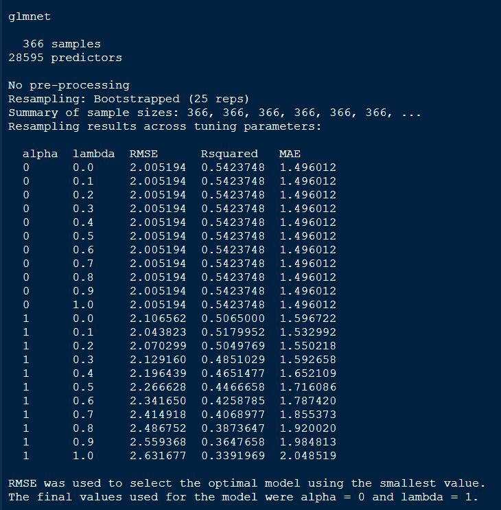
From the above output of the model, we see that alpha = 0, indicating ridge regression was performed in the final model.
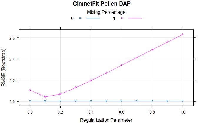
Comparing models: Ridge vs LASSO
plot(glmnetFit_pollen, main = "GlmnetFit Pollen DAP")
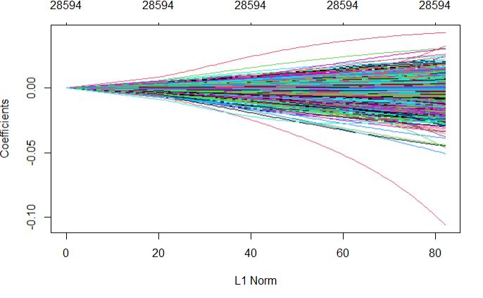
Full regularization path
plot(glmnetFit_pollen$finalModel)
Plot top 20 important variables for Pollen DAP
plot(varImp(glmnetFit_pollen), top = 20)
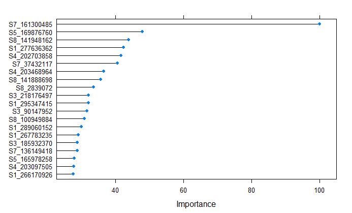
Marker S7_161300485 on chromosome 7 was calculated to be the most important variable by glmnet model for Pollen DAP, which coinsides with one of the major QTL for flowering time in NAM population, that is responsible to vegtative growth and transition from vegitative to reproductive stage.
Validation of glmnet model
Now we can test the robustness of the glmnet model by testing it on test_set data set, and regressing the predicted and measured values.
prediction_glmnet_pollen <- predict(glmnetFit_pollen, test_set)

df_pollen_mes_glmnet <- data.frame(test_set$PollenDAP_BLUPs)
df_pollen_pred_glmnet <- data.frame(prediction_glmnet_pollen)
library(ggplot2)
library(reshape2)

pollen_glmnet_bind <- cbind(df_pollen_mes_glmnet, df_pollen_pred_glmnet)

ggplot(pollen_glmnet_bind, aes(x=test_set.PollenDAP_BLUPs, y=prediction_glmnet_pollen)) +
  geom_point(color="red") + ggtitle("Test set - GLMnet Pollen DAP") +
  geom_smooth(method="lm", se=TRUE, fullrange=FALSE, level=0.95)
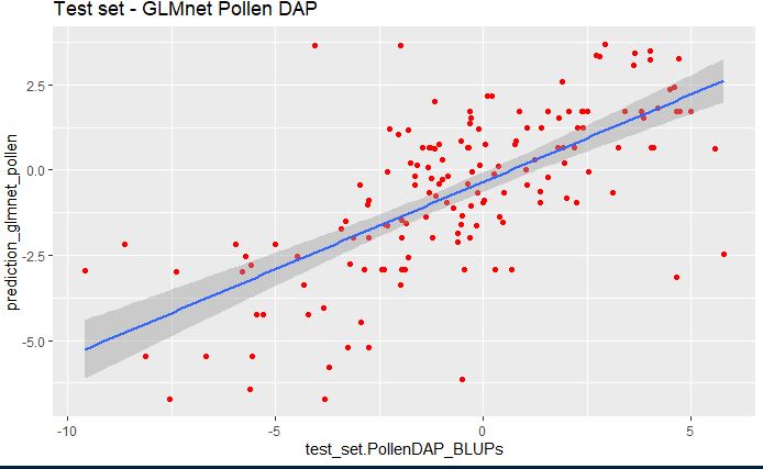
In the above plot, we see that glmnet model pollen predicting the phenotype considerably well.
The RMSE and R-Sq between the predicted and measured values are below:
error_glm_pollen <- prediction_glmnet_pollen - test_set$PollenDAP_BLUPs
rmse_glm_pollen <- sqrt(mean(error_glm_pollen^2))

cat("RMSE of glmnet model for Pollen DAP is", rmse_glm_pollen)
R-squared:
# creat Rsq function
rsq <- function(x, y) summary(lm(y~x))$r.squared

Rsq_Pollen_glmnet <- rsq(test_set$PollenDAP_BLUPs, prediction_glmnet_pollen)

cat("R-squared of glmnet model for Pollen DAP is", Rsq_Pollen_glmnet)
Random forest - rf function
This alogrithm is often acurrate than other algorithms, easier to tune, require less little preprocessing, and capture threshold effects and variable interactions, however, it is less interpretable and often quite slow.
Random forest model
Markers in the column from 2:1942 were used as predictors (x) and the phenotype column as the y variable. Similarly, the performance of the model was evaluated using root mean square error (RMSE) (One can choose other method such as ROC, AUC etc as well), and finally choosing random forest rf as the method in the model.
# Create tunegrid for mtry to tune the model.
tunegrid <- data.frame(.mtry=c(2,4,6, 10, 15, 20, 100))

randomForestFit_pollen = train(x = train_set[7:28601],
                        y = train_set$PollenDAP_BLUPs,
                        method = "rf",
                        metric = "RMSE",
                        tuneGrid = tunegrid
                        )

# print the model output
randomForestFit_pollen
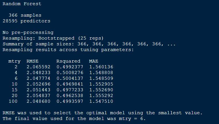
Plotting the randomForestFit for Pollen BLUPs model.
plot(randomForestFit_pollen, main = "Pollen DAP - Random Forest")
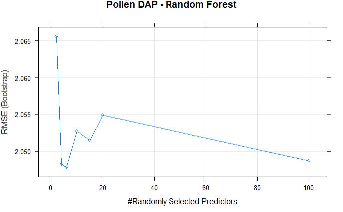
The best mtry with lowest RMSE for this model was 6.
Next, plotting the important predictors based on their calculated importance scores using varImp function.
plot(varImp(randomForestFit_pollen), top = 20)
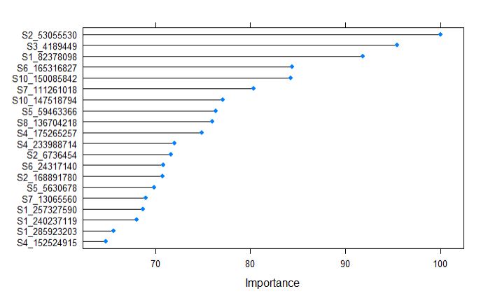
After building the supevised random forest learning model, The top 20 predictors can be ranked by their importance, and from the above plot, we tell that the marker S2_53055530, along with other 6 markers contributing in expalining the variance of the phenotype.
Validation of Random Forest model
Now we can test the robustness of the model by testing it on test_set data set, and regressing the predicted and measured values.
prediction_pollen_rf <- predict(randomForestFit_pollen, test_set)

df_pollen_mes_rf <- data.frame(test_set$PollenDAP_BLUPs)
df_pollen_pred_rf <- data.frame(prediction_pollen_rf)


library(ggplot2);library(reshape2)

pollen_rf_bind <- cbind(df_pollen_mes_rf, df_pollen_pred_rf)

ggplot(pollen_rf_bind, aes(x=test_set.PollenDAP_BLUPs, y=prediction_pollen_rf)) +
  geom_point(color="red") + ggtitle("Test set - Random Forest - Pollen DAP") +
  geom_smooth(method="lm", se=TRUE, fullrange=FALSE, level=0.95)
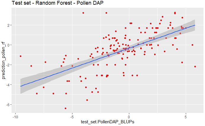
And we can also calculate the RMSE between the predicted and measured values.
error_pollen_rf <- prediction_pollen_rf - test_set$PollenDAP_BLUPs
rmse_pollen_rf <- sqrt(mean(error_pollen_rf^2))

cat("RMSE of Random Forest model for Pollen DAP is", rmse_pollen_rf)
R-squared:
# creat Rsq function
rsq <- function(x, y) summary(lm(y~x))$r.squared

Rsq_Pollen_rf <- rsq(test_set$PollenDAP_BLUPs, prediction_pollen_rf)

cat("R-squared of Random Forest model for Pollen DAP is", Rsq_Pollen_rf)
Comparing the GS models by their type
We can compare the performance of the models by studying their MAE, RMSE and R-squared values side-by-side, making it very convenient.
# Create model_list
model_list_pollen <- list(random_forest = randomForestFit_pollen, glmnet = glmnetFit_pollen)

# Pass model_list to resamples(): resamples
resamples_pollen <- resamples(model_list_pollen)
resamples_pollen

# Summarize the results
summary(resamples_pollen)
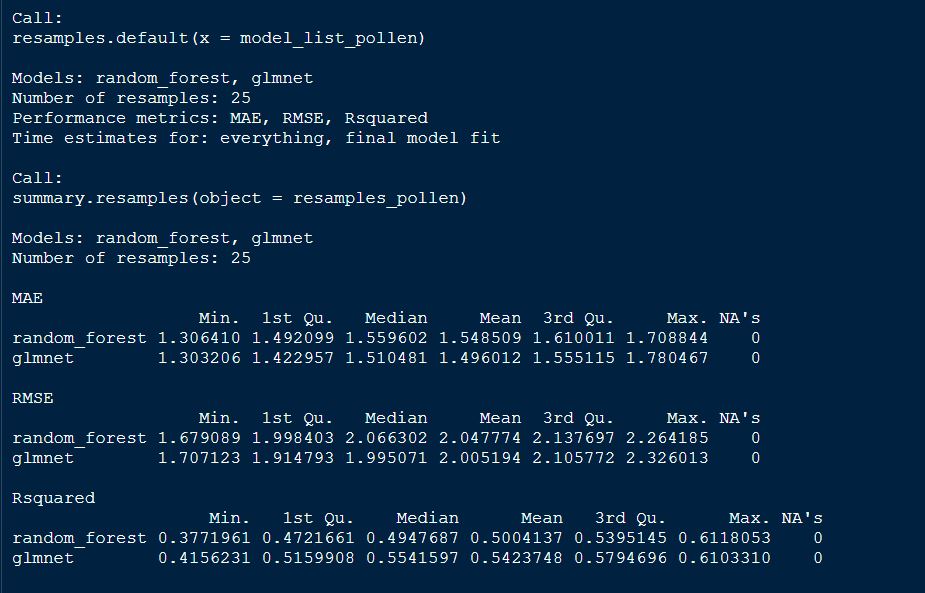
plot both GS models by RMSE
Similarly, we can visually inspect the models accuracies.
par(mfrow=c(1,2))
bwplot(resamples_pollen, metric = "RMSE")
dotplot(resamples_pollen, metric = "RMSE")
par(mfrow=c(1,1))
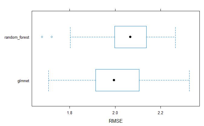
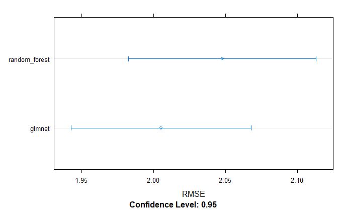
From above table, we can tell that the glmnet model appears to be better model for GS selection of pollen DAP data.
Grain Yield BLUPs
glmnet model
making custom trainControl
myControl <- trainControl(
  method = "cv",
  number =10,
  summaryFunction = twoClassSummary,
  classProbs = T,
  verboseIter = T
)
fitting the model for grain yield using the glmnet model
glmnetFit_yield = train(x = train_set[7:28601],
            y = train_set$yield_BLUPs,
            method = "glmnet",
            metric = "RMSE",
            trainControl = myControl,
            tuneGrid = expand.grid(
              alpha=0:1,
              lambda= 0:10 / 10
            )
          )
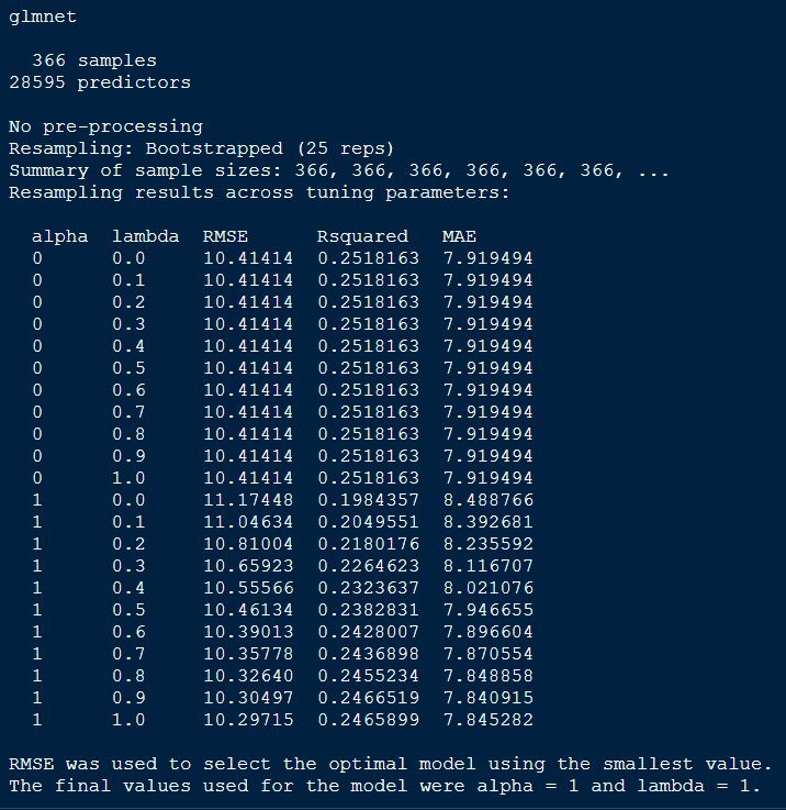
print(glmnetFit_yield)
Comparing models: Ridge vs LASSO
plot(glmnetFit_yield, main = "GlmnetFit Grain Yield")
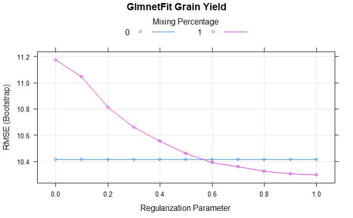
From the above comparison model, we can tell that the alpha and lamda of 1 has lowest RMSE.
Full regularization path
plot(glmnetFit_yield$finalModel)
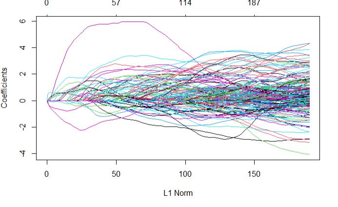
Top predictors
plot(varImp(glmnetFit_yield), top = 20)
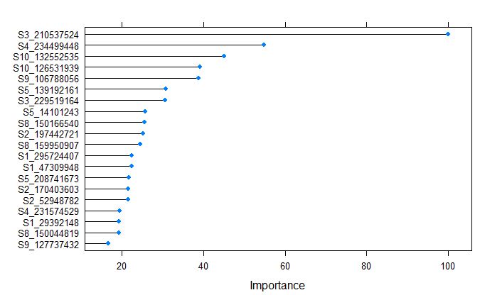
Markers S3_210537524 was calculated as the most important variable by glmnet model.
Validation of glmnet model
Now we can test the robustness of the glmnet model by testing it on test_set data set, and regressing the predicted and measured values.
prediction_glmnet_yield <- predict(glmnetFit_yield, test_set)

df_yield_mes_glmnet <- data.frame(test_set$yield_BLUPs)
df_yield_pred_glmnet <- data.frame(prediction_glmnet_yield)


library(ggplot2);library(reshape2)

yield_glmnet_bind <- cbind(df_yield_mes_glmnet, df_yield_pred_glmnet)

ggplot(yield_glmnet_bind, aes(x=test_set.yield_BLUPs, y=prediction_glmnet_yield)) +
  geom_point(color="red") + ggtitle("Test set - Glmnet - Grain Yield") +
  geom_smooth(method="lm", se=TRUE, fullrange=FALSE, level=0.95)
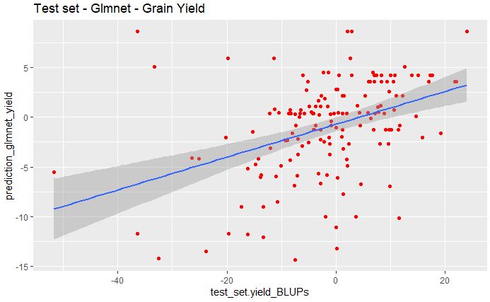
From the above plot, we see poor correlation between the predicted and observed values for grain yield data set.
RMSE and R-Sq between the predicted and measured values.
error_glm_yield <- prediction_glmnet_yield - test_set$yield_BLUPs
rmse_glm_yield <- sqrt(mean(error_glm_yield^2))


cat("RMSE of Glmnet model for Grain yield is", rmse_glm_yield)
R-squared:
# creat Rsq function
rsq <- function(x, y) summary(lm(y~x))$r.squared

Rsq_grain_glmnet <- rsq(test_set$yield_BLUPs, prediction_glmnet_yield)

cat("R-squared of Glmnet model for Grain yield is", Rsq_grain_glmnet)
Random forest model
# Create tunegrid for mtry to tune the model.
tunegrid <- data.frame(.mtry=c(2,4,6, 10, 15, 20, 100))

randomForestFit_yield = train(x = train_set[7:28601],
                        y = train_set$yield_BLUPs,
                        method = "rf",
                        metric = "RMSE",
                        tuneGrid = tunegrid
                        )

# print the model output
randomForestFit_yield
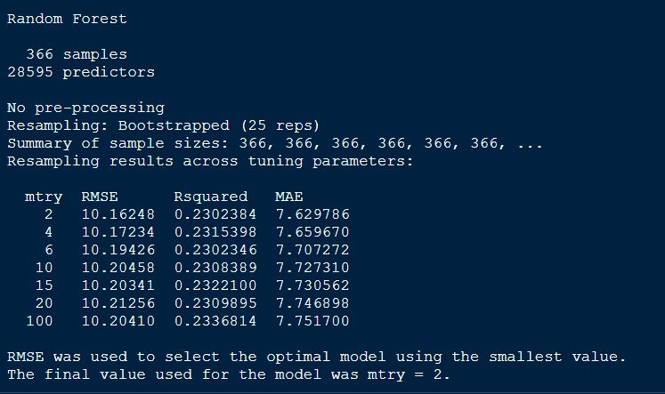
Plotting the randomForetFit model.
plot(randomForestFit_yield, main = "Grain yield - Random Forest")
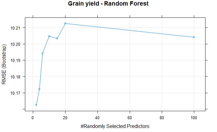
The best mtry with lowest RMSE for this model was 2.
Next, we can plot the important predictors based on their calculated importance scores using varImp function.
plot(varImp(randomForestFit_yield), top = 20)
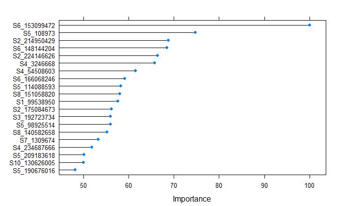
From the above plot, we tell that the S6_153099472 was the most important variable, whch is different from the glmnet model for grain yield.
Validation of Random Forest model
Now we can test the robustness of the model by testing it on test_set data set, and regressing the predicted and measured values.
prediction_yield_rf <- predict(randomForestFit_yield, test_set)

df_yield_mes_rf <- data.frame(test_set$yield_BLUPs)
df_yield_pred_rf <- data.frame(prediction_yield_rf)


library(ggplot2);library(reshape2)

yield_rf_bind <- cbind(df_yield_mes_rf, df_yield_pred_rf)

ggplot(yield_rf_bind, aes(x=test_set.yield_BLUPs, y=prediction_yield_rf)) +
  geom_point(color="red") + ggtitle("Test set - Random Forest - Grain Yield") +
  geom_smooth(method="lm", se=TRUE, fullrange=FALSE, level=0.95)
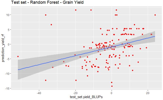
Similar to glmnet model, random forest fail to predict the grain yield.
And we can also calculate the RMSE between the predicted and measured values.
error_yield_rf <- prediction_yield_rf - test_set$yield_BLUPs
rmse_yield_rf <- sqrt(mean(error_yield_rf^2))


cat("RMSE of Random Forest model for Grain yield is", rmse_yield_rf)
R-squared:
# creat Rsq function
rsq <- function(x, y) summary(lm(y~x))$r.squared

Rsq_grain_rf <- rsq(test_set$yield_BLUPs, prediction_yield_rf)

cat("R-squared of Random Forest model for Grain yield is", Rsq_grain_rf)
Comparing the GS models by their type
We can compare the performance of the models by studying their MAE, RMSE and R-squared values side-by-side, making it very convenient.
# Create model_list
model_list_yield <- list(random_forest = randomForestFit_yield, glmnet = glmnetFit_yield)

# Pass model_list to resamples(): resamples
resamples_yield<- resamples(model_list_yield)
resamples_yield

# Summarize the results
summary(resamples_yield)
plot both GS models by RMSE
Similarly, we can visually inspect the models accuracies.
par(mfrow=c(1,2))
bwplot(resamples_yield, metric = "RMSE")
dotplot(resamples_yield, metric = "RMSE")
par(mfrow=c(1,1))
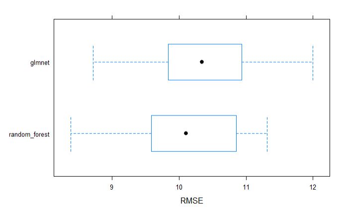
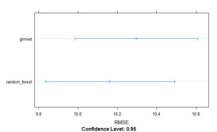
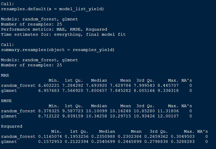
From above table, we can tell that the random forest model appears to be slighlty better model incoparison to glmnet for grain yield.
4.0 Summary of genomic selection algorithms on selected traits
| Trait | Model | Set | RMSE | R-Sq |
|---|---|---|---|---|
| Pollen DAP | Glmnet | Training set | 2.01 | 0.54 |
| Test set | 2.28 | 0.39 | ||
| Random forest | Training set | 2.04 | 0.50 | |
| Test set | 2.37 | 0.40 | ||
| Grain yield | Glmnet | Training set | 10.3 | 0.25 |
| Test set | 10.75 | 0.16 | ||
| Random forest | Training set | 10.2 | 0.23 | |
| Test set | 11.08 | 0.12 |
In summary, Pollen DAP trait had a high heritability, and both GS models had a relatively statisfactory prediction accuracy in both training and test data sets. In contrast, grain yield had moderate heriatblity indicating significant influence of genetic and environmental componets on this trait, and both GS models built with only genomic markers failed, which tells us that heritability of a trait is an important characteristics as so are the environmental components. Therefore, its strongly advised to calculate the heritability of trait of interest prior to building any GS model, so that one has idea of what to expect from the GS model performance.
References
McFarland, B.A., AlKhalifah, N., Bohn, M., Bubert, J., Buckler, E.S., Ciampitti, I., Edwards, J., Ertl, D., Gage, J.L., Falcon, C.M. and Flint-Garcia, S., 2020. Maize genomes to fields (G2F) : 2014–2017 field seasons: genotype, phenotype, climatic, soil, and inbred ear image datasets. BMC Research Notes, 13(1), pp.1-6.