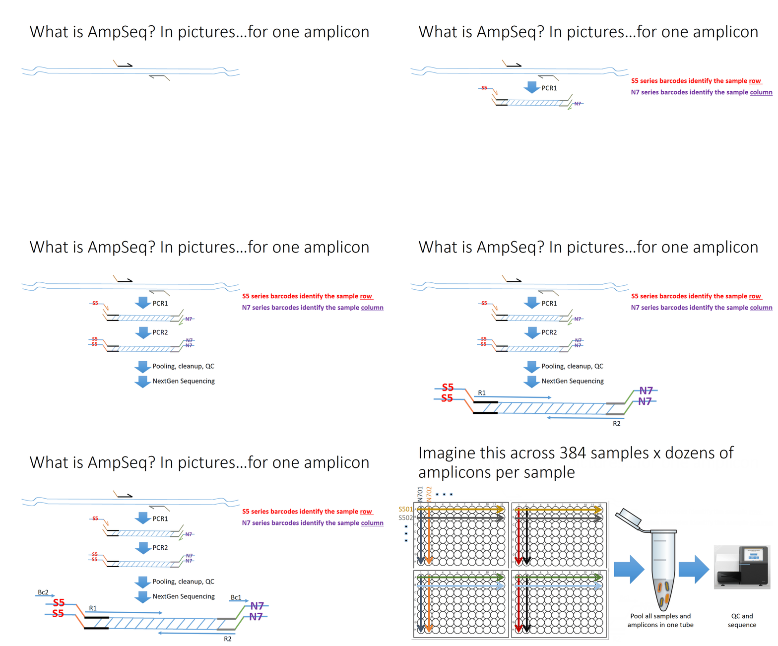
Amplicon Sequencing (AmpSeq) technology combines highly multiplexed PCR sequences of multiple barcoded samples in a single reaction. Amplicons include SNP, haplotypes, SSRs and presence/absence variants. Currently, in a single reaction about 400 amplicons and 3000 samples can be processed simultaneously. In this blog, my goal is to basically introduce the concept and analysis of AmpSeq data. For further descriptive information on AmpSeq, please read the AmpSeq paper by Yang et al 2016 at thislink .
AmpSeq in pictures
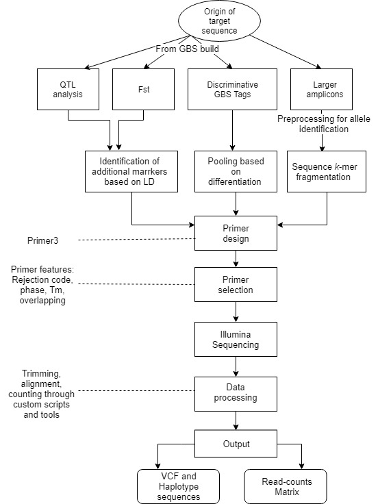
Flowchart of the steps involved in the AmpSeq process

Effect of poor DNA quality or quantity?
- DNA quantity is not important, works with <1 ng/uL
- Poor DNA quality could cause missing data.
- If you can see amplification in a gel, then primer and template are outstanding. (You will get data even for amplicons that are not visible on a gel.)
Primer transferability across species?
- Amplicons have some degree of species specificity.
- Best to design primers specific to target organism, but in the absence of existing reference, you may get useful information.
What are some applications of AmpSeq
- Marker conversion
- Marker assisted selection
- Population genetics
- Organellar genetics
- Candidate gene profiling
- Mutation detection
- Metagenomics
Any marker with a sequence basis can be converted to AmpSeq (eg here, simple sequence repeat, SSR)

Interpreting the above figure: by electrophoresis, the top 5 alleles would all appear to be the same SSR allele.
1)Two of the SNPs shown here occur with multiple SSR allele sizes.
2)Excellent quality data from undetectable quantities of dirty DNA.
3)Analysis of same DNA by SSR capillary electrophoresis was a mess.
what are the pros and cons of AmpSeq?
Pros
- Discover, convert, and genotype in one platform
- Many uses
- Low cost, high multiplexing, low missing data*
- Can combine unrelated projects, save $$
- Poor DNA is fine
- Can re-analyze old DNA
- Primer optimization not required
- Data analysis semi-automated
- Moderate turnaround (2-4 weeks)
Cons
- Presence/absence markers: overlapping read count distributions
- NTC Blank wells with data
- SNP markers: genotype-dependent amplification of alleles
- 10% of reads from off-target amplification
- Uneven read depth
- 15-30% of non-validated primers will fail
- Highly multiplexed PCR setup works best with liquid handler
- Bioinformatics requirement
Note: Gene walking: Overlapping amplicons return only the shortest product. Overlapping primers will self-amplify. High efficiency primers will use a lot of data. Avoid at primer design OR amplify separately then pool for sequencing
How to design AmpSeq primers?
The easy way:
- Use existing primers that work well, OR design new locus-specific primers using Primer3.
- Add forward/reverse linkers
GBS marker conversion (Horticulture Research 3: 16002)
- SNP haploblock spanning QTL
- Presence/Absence tag
Now your received your AmpSeq data, whats next?!?
AmpSeq data analysis is a semi-automated computational pipeline. One may consult the Jonathan Fresendo’s Github page for the pipeline scripts and commands used for Primer Design, SNP calling, and Haplotyping at this link https://github.com/JFresnedo/AmpSeq
Analyzing the AmpSeq data with analyze_amplicon.pl pipeline
Now, I would like to introduce the pipeline analyze_amplicon.pl used in the analysis of paired-end AmpSeq data. This tutorial is divided into the following Steps:
STEP 1. Preparing Key File andSample file
STEP 2. Running the script analyze_amplicon.pl
STEP 3. Output and data interpretation
STEP 1. Preparing Key File, Sample file and Sample Read Files
Key File
A two-column, tab separated text file (key_file.txt) listing the primer names (ending _F and _R to indicate forward and reverse primer) and primer sequences. Creating this file is a straightforward, for which having the sequences of the primers is enough, however, it is important that one removes all forward and reverse linker sequences from individual primer sequences in the key file. The naming of primer sequences maybe somewhat arbitrary, but it is always better to use intuitive names for downstream analysis. The file is simple and should not have a header.
Below is an example of the key file key_file.txt:
Ren1_S13_20430245_F	TTAGGAGATAGGCCTGGACAAG
Ren1_S13_20430245_R	TTTCCTTGCAGCCAAACAGACG
Ren1_SC47_6_F	GATCAGCCACCAAAAGAGGA
Ren1_SC47_6_R	GCTTTGTAGTCTGCCTACTTGATG
Ren6_PN9_063_F	TCCTAAGACAAAGTTCCCTTCA
Ren6_PN9_063_R	GTTACAGTTGAATCCTTGCACA
Ren6_PN9_068_F	CCCCAATCTTAAATGGAACA
Ren6_PN9_068_R	TAGTGGGACGTTGGACACTT
Ren7_PN19_018_F	CAAAACAAGTCCATTGCGTTTA
Ren7_PN19_018_R	TGTCCCATGACAGTTTATCCAG
Ren7_VVin74_F	TTGGTTGAGGGAAAAAGGAAAG
Ren7_VVin74_R	AAGAAATATGAGGTTGGGTGAG
Ren7_VVIu09_F	TATCCTCTGTCACATTAGTTGT
Ren7_VVIu09_R	GTGATATTTTCCCGTTGTTAGG
Rpv12_UDV014_F	TGAAAGTCGATGGAATGTGC
Rpv12_UDV014_R	TTGCATCTCCCTTCTCAATG
Rpv12_UDV370_F	TGGTTGAGCACAGTTCTTGG
Rpv12_UDV370_R	CAGAAAGCCCTGATCTCCTG
Run1_CB3334_Haplo64_F	CCAAGGTGCAGATAATGAAAGAA
Run1_CB3334_Haplo64_R	GGTAGTCTTTCGTGTGCATATTT
Sample file
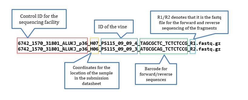
Fastq files from sequencing having epithets R1 and R2 indicates that pair-ended sequencing was performed; At the Cornell University sequencing facility read files are named as in below example:
The sample file is a .txt file. When you get the names directly from the sequencing files, it may be tricky to prepare the files, but if you are handy with Excel and know how to delimit separation, using find and replace function, and concatenation, the task is simple. To help you with that a good starting point is to have a list of the fastq files located in the directory tutorial, for that you use:
ls *fastq.gz > genotypes.txt
And from that list you can develop sample file that looks like below:
Parent1_B10	Parent1_B10_R1.fastq.gz	Parent1_B10_R2.fastq.gz
Parent2_C12	Parent2_C12_R1.fastq.gz	Parent2_C12_R2.fastq.gz
Progeny01_H01	Progeny01_H01_R1.fastq.gz	Progeny01_H01_R2.fastq.gz
Progeny02_F02	Progeny02_F02_R1.fastq.gz	Progeny02_F02_R2.fastq.gz
Progeny03_G02	Progeny03_G02_R1.fastq.gz	Progeny03_G02_R2.fastq.gz
Progeny04_H02	Progeny04_H02_R1.fastq.gz	Progeny04_H02_R2.fastq.gz
Progeny05_A03	Progeny05_A03_R1.fastq.gz	Progeny05_A03_R2.fastq.gz
Progeny06_B03	Progeny06_B03_R1.fastq.gz	Progeny06_B03_R2.fastq.gz
Progeny07_C03	Progeny07_C03_R1.fastq.gz	Progeny07_C03_R2.fastq.gz
Progeny08_D03	Progeny08_D03_R1.fastq.gz	Progeny08_D03_R2.fastq.gz
Progeny09_E03	Progeny09_E03_R1.fastq.gz	Progeny09_E03_R2.fastq.gz
Progeny10_F03	Progeny10_F03_R1.fastq.gz	Progeny10_F03_R2.fastq.gz
In the sample file, column 1 contains the IDs can be specified by the user, but it is recommended that the names keep the coordinate of the well (e.g. H01, A03, D03) for quality control and particularly when genotypes (plants) are duplicated in the plate. Columns 2 and 3 are the names of the two fastq files retrieved from the sequencer, therefore, these names use the convention of naming by the Cornell sequencing facility (lane, plate, ID, well), and the names need to conserve at least R1 or R2.fasq.gz . Finally, save the file as a text (.txt) file.
STEP 2. Running the script analyze_amplicon.pl
Place the individual fastq files, the key_file and sample_file in a directory using FileZilla (instruction on how to transfer at this link https://wiki.filezilla-project.org/Using ).
Note: Normally, it is strongly suggested to make copies all the original fastq files (sample read files) in a backup folder.
Then, from the directory, one is able to run the script analyze_amplicon.pl by typing the following command line on the Linux console:
$analyze_amplicon.pl –i 8 –s sample_file.txt –k key_file.txt –o Output –m clustalo:clustal
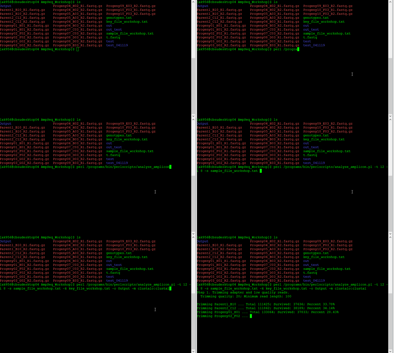
To list all the parameters in the script analyze_amplicon.pl please type the following on your Linux command line console:
/programs/bin/perlscripts/analyze_amplicon.pl –h
Output:
-o: outdir
-s: Sample file name
-k: Key file name
-y: mismatches in primer matching (number, default 0)
-z: remove both primers from haplotypes (y or n, default n)
-i: skip steps. (steps are specified below.)
-d: parameter for trimming reads, using 2 numbers separated by ':'. 205 Default: 20:100. They are: quality score:minimum_read_length
-n: fasta file of adapter sequence, default is the i7 i5 adapter file 207 /programs/Trimmomatic-0.36/adapters/amplicon-SE.fa
-w: running modes for paired end reads. 1(default).contig the overlapped 209 reads, discard the reads that do not form contig; 2.concatenate the two 210 reads using reads length defined by -l option, the reverse reads is 211 reverse complemented; 3. mixed mode, contig the reads, and concate reads 212 that do not contig
-l: switch to concatenate reads mode. Truncate read to specified length 214 then concatenate
-v: parameter for contiging, using 3 numbers separated by ':'. Default: 216 20:250:0.05. They are: minimum_overlap:max_overlap_length:mismatch_rate
-u: parameter for contiging, allow outie
-b: the length of F primer used for identify a locus in the sequence 219 reads, default: the shortest primer length
-c: minimum copies for an haplotype across samples, default:2
-r: reference sequence
-x: filter haplotype by alignment to reference. e.g. -x 50:85:90, 223 alignment with 50nt 5' sequence, 85% of the 50nt can be aligned, 90% 224 identical in in aligned region.
-a: minimum ratio of read count between the two haplotypes (low/high 226 default: 0.2)
-m: Specify the multiple sequence alignment software, format, and 228 length per line, separated by : (e.g. clustalw:[CLUSTAL, GCG, GDE, 229 PHYLIP, PIR, NEXUS, FASTA], or clustalo:[fasta, 230 clustal,msf,phylip,selex,stockholm,vienna]:10000). Default: not 231 generated.
-j: number of simultaneous jobs
-t: computing threads
-h: print help
Using the default parameters which includes skipping step 8, the processing of data depends on samples and number of markers. From your terminal you will see a lot of information according to the step being ran, for example:
For step 1: during this step the sequencing information is trimmed for the adaptors and keeping reads with a minimum quality. The trimming quality and the quality threshold of the reads may be defined by the use with the option -d.
Step 1. Trimming adapter and low quality reads.
  Trimming quality: 20; Minimum read length: 100

Trimming Parent1_B10 ... Total 111425; Survived: 37693; Percent 33.83%
Trimming Parent2_C12 ... Total 111862; Survived: 38246; Percent 34.19%
Trimming Progeny01_H01 ... Total 133064; Survived: 37891; Percent 28.48%
Trimming Progeny02_F02 ... Total 87129; Survived: 18887; Percent 21.68%
Trimming Progeny03_G02 ... Total 135088; Survived: 43731; Percent 32.37%
Trimming Progeny04_H02 ... Total 122080; Survived: 25971; Percent 21.27%
Trimming Progeny05_A03 ... Total 131967; Survived: 41960; Percent 31.80%
Trimming Progeny06_B03 ... Total 122834; Survived: 34413; Percent 28.02%
Trimming Progeny07_C03 ... Total 104262; Survived: 25745; Percent 24.69%
Trimming Progeny08_D03 ... Total 118236; Survived: 33469; Percent 28.31%
Trimming Progeny09_E03 ... Total 120362; Survived: 33234; Percent 27.61%
Trimming Progeny10_F03 ... Total 91115; Survived: 15923; Percent 17.48%
Read trimming finished.
For step 2: in this step a consolidation of the reads is performed and can be made in three different ways (modes). The definition of the mode to use may be entered through the option and -l.
Step 2. Contiging (mode 1) the overlapping read pairs. Discard the non-overlapping reads.
  Range of overlap: 20 bp - 250 bp; Mismatch rate: 0.03
Contiging read pair for Parent1_B10 ... Total:  37693; Form contig: 98.83%
Contiging read pair for Parent2_C12 ... Total:  38246; Form contig: 99.24%
Contiging read pair for Progeny01_H01 ... Total:  37891; Form contig: 99.27%
Contiging read pair for Progeny02_F02 ... Total:  18887; Form contig: 99.38%
Contiging read pair for Progeny03_G02 ... Total:  43731; Form contig: 99.17%
Contiging read pair for Progeny04_H02 ... Total:  25971; Form contig: 99.32%
Contiging read pair for Progeny05_A03 ... Total:  41960; Form contig: 99.10%
Contiging read pair for Progeny06_B03 ... Total:  34413; Form contig: 99.13%
Contiging read pair for Progeny07_C03 ... Total:  25745; Form contig: 99.25%
Contiging read pair for Progeny08_D03 ... Total:  33469; Form contig: 98.86%
Contiging read pair for Progeny09_E03 ... Total:  33234; Form contig: 99.06%
Contiging read pair for Progeny10_F03 ... Total:  15923; Form contig: 99.16%
Read assembly/concatenate finished.
For step 3: the reads identified in the sequence files are split based on the sequences of the forward primer (from key_file.txt). The length of the primer informs the minimum overlapping to consider and it may be modified by the use using the option -b.
Step 3. Splitting sequences files by locus using primer F.
  Forward primer length:  20 to 23
  Use shortest primer length  20 bp to split locus in  sequence file
  Reverse primer length:  20 to 24
  Use shortest primer length  20 bp to split locus in  sequence file
Parent1_B10     Total: 37228    Unmatched_F: 15050      Unmatched_R: 966
Parent2_C12     Total: 37945    Unmatched_F: 4311       Unmatched_R: 1451
Progeny01_H01   Total: 37580    Unmatched_F: 5895       Unmatched_R: 1261
Progeny02_F02   Total: 18744    Unmatched_F: 4929       Unmatched_R: 566
Progeny03_G02   Total: 43336    Unmatched_F: 16116      Unmatched_R: 1086
Progeny04_H02   Total: 25764    Unmatched_F: 3683       Unmatched_R: 873
Progeny05_A03   Total: 41555    Unmatched_F: 18370      Unmatched_R: 915
Progeny06_B03   Total: 34083    Unmatched_F: 13639      Unmatched_R: 876
Progeny07_C03   Total: 25520    Unmatched_F: 4092       Unmatched_R: 838
Progeny08_D03   Total: 33039    Unmatched_F: 9190       Unmatched_R: 984
Progeny09_E03   Total: 32882    Unmatched_F: 13038      Unmatched_R: 830
Progeny10_F03   Total: 15763    Unmatched_F: 2541       Unmatched_R: 536
File splitting finished!
For step 4: in this step the reads that are identical in sequences are grouped by sample (i.e. ID in the sample_file.txt).
Step 4. Collapsing identical reads in each sample
Collapsing reads for sample Parent1_B10 ...
Collapsing reads for sample Parent2_C12 ...
Collapsing reads for sample Progeny01_H01 ...
Collapsing reads for sample Progeny02_F02 ...
Collapsing reads for sample Progeny03_G02 ...
Collapsing reads for sample Progeny04_H02 ...
Collapsing reads for sample Progeny05_A03 ...
Collapsing reads for sample Progeny06_B03 ...
Collapsing reads for sample Progeny07_C03 ...
Collapsing reads for sample Progeny08_D03 ...
Collapsing reads for sample Progeny09_E03 ...
Collapsing reads for sample Progeny10_F03 ...
For step 5: in the step the grouped files are collapsed according to the names of the loci that one have provided in the key_file.txt thus, now it is possible to have read counts in by locus-sample bases.
Step 5. Collapsing reads across all samples.
Collapsing gene Ren1_S13_20430245 ...
Collapsing gene Ren1_SC47_6 ...
Collapsing gene Ren6_PN9_063 ...
Collapsing gene Ren6_PN9_068 ...
Collapsing gene Ren7_PN19_018 ...
Collapsing gene Ren7_VVin74 ...
Collapsing gene Ren7_VVIu09 ...
Collapsing gene Rpv12_UDV014 ...
Collapsing gene Rpv12_UDV370 ...
Collapsing gene Run1_CB3334_Haplo64 ...
Collapsing identical sequences per locus finished.
For step 6: In this step is the consolidation in by locus-sample bases of the information recovered in step 5 and which will be stored in different forms and formats for subsequent analyses.
Step 6. Making haplotype-by-sample matrix for each locus.
process gene Ren1_S13_20430245 ...
Warning: Ren1_S13_20430245 file test/merged/Ren1_S13_20430245 is empty.
process gene Ren1_SC47_6 ...
process gene Ren6_PN9_063 ...
process gene Ren6_PN9_068 ...
process gene Ren7_PN19_018 ...
process gene Ren7_VVin74 ...
process gene Ren7_VVIu09 ...
process gene Rpv12_UDV014 ...
process gene Rpv12_UDV370 ...
process gene Run1_CB3334_Haplo64 ...
Warning: Run1_CB3334_Haplo64 file test/merged/Run1_CB3334_Haplo64 is empty.
Making haplotype-by-sample table finished.
For step 7: this step ends with a file called hap_genotype, which has the information of the two most repeated haplotypes (per locus) observed across the samples analyzed, the data is provided for every sample in a format similar to a VCF file. The number of haplotypes to report may be modified by the user by using the option -c. The options -x -a and -m are of relevance for this step too, and the user may play with these options to be more conservative or liberal about the determination of the top distinct haplotypes.
Step 7. Identifying top 2 haplotypes from each sample.
Identifying top 2 haplotypes finished.
And finally for step 8: this step is not relevant for the current analysis. However, it may be really important for some applications. Particularly, if you know the exact sequence of the amplicon that you are analyzing, through this step one will be able to call SNPs within the amplicon sequence. Let’s say that you are going to analyze specific gene sequences for which SNPs or Indels will give you additional insights about the variants that are explaining particular phenotypes. In order to use this option you need to provide a fasta file having the sequences of the target amplicons and provide the name of the file in front of the option -r. The names of the sequences in the fasta file must match with the name of the primers used to amplify that sequence. If you do not know the sequence of the amplicon, the analysis of amplicons as in this example will help to unravel the sequences flanked for markers and which may be useful to determine target sequences for subsequent studies for the identification of variants.
Step 8. Calling SNP skipped!
STEP 4. Output and data interpretation
The output of this data processing is located in the directory Output, which has the following directories and files:
cd ..
ls -R
.:
assemble
collapse
hap_genotype
haplotype2fasta
haplotype2sample_raw
merged
runlog
split
stats
tmp
trimmed
vcf
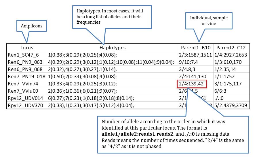
The directories and files are showed above: runlog corresponds to a file tacking all the procedures and output ran during the process (It is very important to check this file if the quality of the data is a concern). hap_genotype is one of the most relevant files from this analysis, and in a format similar to a VCF it shows the information about the two most important haplotypes (which can also be interpreted as alleles) of every amplicon in every ID sample.
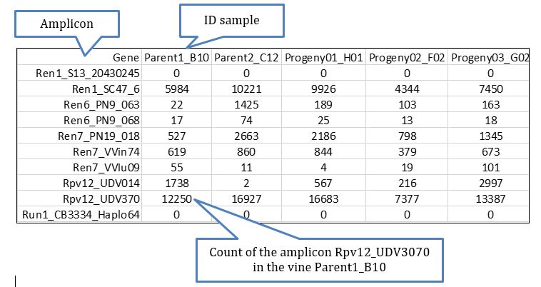
For the purpose of this analysis, the most important file to check first is gene_sample_read_count.txt located in Output/stats/ and which inform about the read counts per amplicon per sample. This file is easily handled using Excel, which allows to add phenotypic information available for the samples and thus to perform some routines to define the most relevant amplicons for the exhibition of the phenotype based on logistic regression.
An excerpt of the file with phenotypic is shown below:
A file that can be of interest for certain projects in which the knowledge of the genotypes (understood as diplotypes for the observed dominant haplotypes/alleles) per sample of certain amplicons is highly relevant, perhaps the most informative file is hap_genotype which shows the genotype for every individual based on the dominant haplotypes identified in the data process, the data retrieved looks like more or less like this:
Convert your Halpotype results into VCF
To create a VCF from the haplotype calls or to run the step 8, you need a reference genome; this step will fail without it. The easy way to make a VCF file from your haplotype calls is to use this another script called Haplotype_to_VCF.pl, it can be downloaded at this Link
Before you convert your halpotypes to VCF, I suggest looking at the parameters first by typing and running it shown below:
                perl halplotype_to_VCF.pl -h

                -g: Input genotype file
                -f: minimum allele frequency
                -b: define blank samples index, if there are several separated by comma. First sample index is 1.
                -m: maternal parent index, if there are several separated by comma. First sample index is 1.
                -p: paternal parent index, if there are several separated by comma. First sample is 1.
                -n: family name
                -h: help menu.
Finally, you can run the script shown in the example below:
perl haplotype_to_VCF.pl -g hap_genotype -f 0.05 -n Family_name
This will create two files: the VCF and allele lookup file – its an important file for any downstream analysis, which contains haplotype IDs and their assigned pseudo ACGT alleles that can be used to find the associated haplotype sequences. However, in case your markers do not have chromosome names and their physical positions, you will have to make a “fake” CHROM and POS column in excel. See the screenshot below:

--- End of Tutorial ---
Thank you for reading this tutorial. I really hope this helpful in giving you the concept and technology behind AmpSeq and the data analysis. If you have any questions or comments, please let comment below or send me an email. Happy AmpSeq-ing !
Bibliography
Computational analysis of AmpSeq data for targeted, high-throughput genotyping of amplicons Fresnedo-Ramírez, Jonathan, Shanshan Yang, Qi Sun, Avinash Karn, Bruce I. Reisch, and Lance Cadle-Davidson. Frontiers in plant science 10 (2019): 599.
