In this tutorial, I used two popular machine learning algorithms: Random Forest and GLMnet for Genomic Prediction of a quantitative trait. There are several machine learning R packages available, however, in this tutorial i used caret package. The objective was to develop two models: Random forest and glmnet using real data sets consisting genetic markers, that were used as predictors to predict a quantitative trait (names of the variables were disguised in this tutorial), and finally, comparing the performance of the two models by testing them on a validation set.
Data preparation
Step 1. libraries and set seed
library(randomForest)
library(mlbench)
library(caret)
library(e1071)

set.seed(06252020)
Step 2. Load input file and explore
The genetic marker data was converted into numeric format. One can use TASSEL software to convert their data into numeric format, as well as numerically impute any sites with missing data. Please remember, its curicial to impute the data or else it will result an error while executing the model and or result biased model output. Additionally, I removed any missing phenotypic values from the data set.
Download the dataset i used in this tutorial here at this link: Click here
Code:
phenoGeno <- read.table("rhGeno_numericImpu_malateBlues_HI.txt", header = T, na.strings = "NA")

## Explore the data
head(phenoGeno)
tail(phenoGeno)
Output:
   phenotype marker1 marker2 marker3 marker4 marker5 marker6 marker7 marker8
 1  3.301974     0.5     0.0     0.5     0.0     0.0   0.500       1     0.0
 2  3.314499     0.0     0.0     1.0     0.0     0.0   1.000       1     0.0
 3  4.701069     0.5     0.0     1.0     0.0     0.0   0.500       1     0.0
 4  4.943334     1.0     0.5     0.5     0.5     0.5   0.252       1     0.5
 5  5.061315     0.0     0.0     1.0     0.0     0.0   0.500       1     0.0
 6  5.144740     0.5     0.0     0.5     0.0     0.0   1.000       1     0.0
Step 2.1 Distribution of the phenotype data
hist(phenoGeno$phenotype)
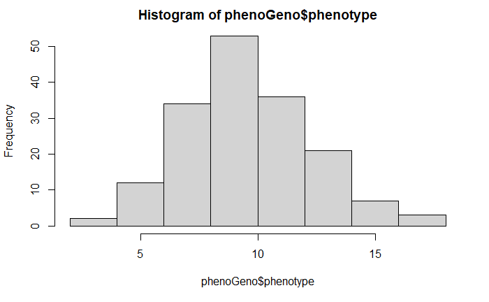
The phenotype data is normally distributed, and no preprocessing was performed. However, I do suggest transforming the data if required.
Step 3. Training and Test set
Step 3.1 Splitting the data into train and test set
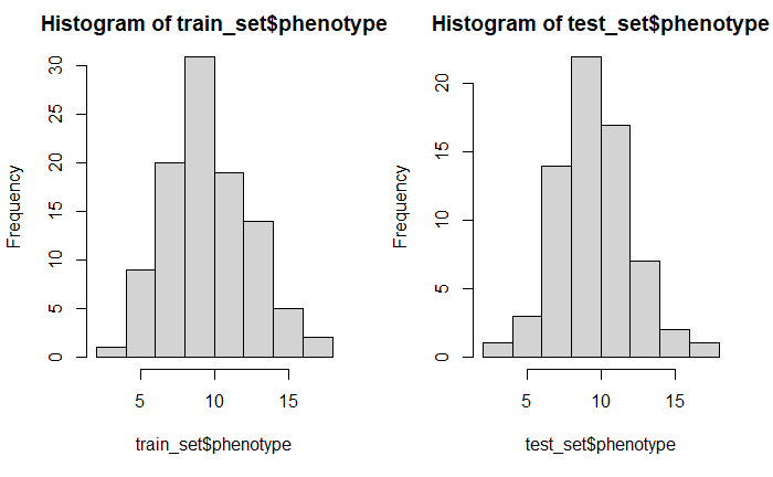
In the next step, the imported data was split into 60/40 split, since the dataset i have used in this tutorial is small and, therefore, 60/40 gives a larger and more reliable test set.
Step 3.2 Randomizing the order of the dataset
rows <- sample(nrow(phenoGeno))

phenoGeno <- phenoGeno[rows, ]

head(phenoGeno)

Step 3.3 Find the rows to split
For this tutorial, data will be split into 60/40, which provides a larger and more reliable test/validation set.
split <- round(nrow(phenoGeno) * 0.60)

train_set <- phenoGeno[1:split,]

test_set <- phenoGeno[(split + 1):nrow(phenoGeno),]
Step 3.4 Confirm train and test set sizes
# Check the ratios of training and test sets
nrow(train_set)/nrow(phenoGeno)

nrow(test_set)/nrow(phenoGeno)

# plot the two data sets
par(mfrow=c(1,2))
hist(train_set$phenotype)
hist(test_set$phenotype)
par(mfrow=c(1,1))
Random forest - rf function
The name Random forest is a popular name in the area of machine learning. This alogrithm is often acurrate than other algorithms, easier to tune, require less little preprocessing, and capture threshold effects and variale interactions, however, it is less interpretable and often quite slow.
TrainControl object
Before creating and running the models, its a good idea to create a trainControl object to tune parameters and further control how models are created.
myTrainingControl <- trainControl(method = "cv",
                              number = 10,
                              savePredictions = TRUE,
                              classProbs = TRUE,
                              verboseIter = TRUE)
Creating the model
Markers in the column from 2:1942 were used as predictors (x) and the phenotype column as the y variable. Similarly, the performance of the model was evaluated using root mean square error (RMSE) (One can choose other method such as ROC, AUC etc as well), and finally choosing random forest rf as the method in the model.
Code:
# Create tunegrid for mtry to tune the model.
tunegrid <- data.frame(.mtry=c(2,4,6, 10, 15, 20, 100))

randomForestFit = train(x = train_set[2:1942],
                        y = train_set$phenotype,
                        method = "rf",
                        metric = "RMSE",
                        tuneGrid = tunegrid
                        )

# print the model output
randomForestFit
Output:
 Random Forest

  101 samples
 1941 predictors

 No pre-processing
 Resampling: Bootstrapped (25 reps)
 Summary of sample sizes: 101, 101, 101, 101, 101, 101, ...
 Resampling results across tuning parameters:

   mtry  RMSE      Rsquared   MAE
     2   2.754033  0.1057086  2.233488
     4   2.736635  0.1023974  2.221954
     6   2.717262  0.1151134  2.203889
    10   2.710155  0.1121776  2.200923
    15   2.700049  0.1159634  2.197863
    20   2.700378  0.1109506  2.194062
   100   2.668136  0.1296488  2.159293

 RMSE was used to select the optimal model using the smallest value.
 The final value used for the model was mtry = 100.
Plotting the randomForetFit model.
plot(randomForestFit, main = "Random Forest")
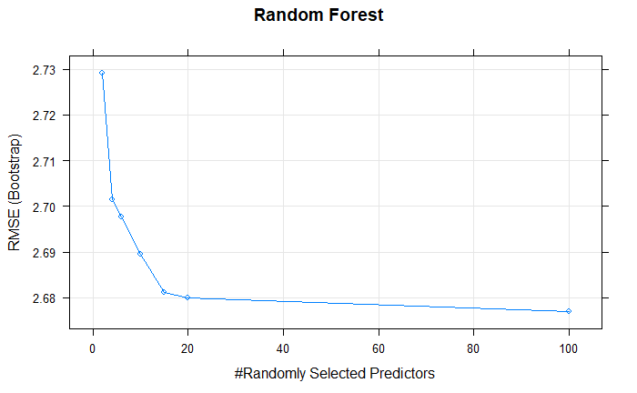
The best mtry with lowest RMSE for this model was 10.
Next, we can plot the important predictors based on their calculated importance scores using varImp function.
plot(varImp(randomForestFit), top = 20)
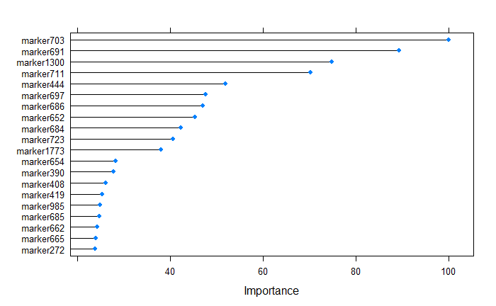
After building the supevised random forest learning model, The top 20 predictors can be ranked by their importance, and from the above plot, we tell that the marker703 was the most important variable.
Validation of Random Forest model
Now we can test the robustness of the model by testing it on test_set data set, and regressing the predicted and measured values.
prediction_rf <- predict(randomForestFit, test_set)

plot(test_set$phenotype, prediction_rf,
     main = "Random Forest", pch=17, col=c("red"))
abline(lm(prediction_rf~test_set$phenotype))
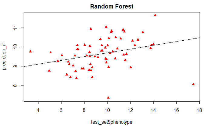
And we can also calculate the RMSE between the predicted and measured values.
error_rf <- prediction_rf - test_set$phenotype
rmse_rf <- sqrt(mean(error_rf^2))
rmse_rf
Glmnet model - glmnet function
This is another popular machine learning algorithm, which has some benefits over the Random forest model. It is a extension of glm models with a built-in variable selection that also help in dealing with collinearity and small sizes. The glmnet has two primary froms: 1) LASSO regression, which penalizes number of non-zero coefficients, and 2) Ridge regression, which penalizes absolute magnitude of coefficients. It also attempts to find a parsimonious aka simple model and pairs well with random forest models.
First, we create the glmnet models, which is a combination of lasso and ridge regression, and we can fit the mix of the two models by selecting the values for alpha and lambda, as shown in the below code snippet.
glmnet model
Code:
glmnetFit = train(x = train_set[2:1942],
            y = train_set$phenotype,
            method = "glmnet",
            metric = "RMSE",
            trainControl = myControl,
            tuneGrid = expand.grid(
              alpha=0:1,
              lambda= 0:10 / 10
            )
          )

print(glmnetFit)
Output:
 glmnet

  101 samples
 1941 predictors

 No pre-processing
 Resampling: Bootstrapped (25 reps)
 Summary of sample sizes: 101, 101, 101, 101, 101, 101, ...
 Resampling results across tuning parameters:

   alpha  lambda  RMSE      Rsquared    MAE
   0      0.0     2.724706  0.13509467  2.256743
   0      0.1     2.724706  0.13509467  2.256743
   0      0.2     2.724706  0.13509467  2.256743
   0      0.3     2.724706  0.13509467  2.256743
   0      0.4     2.724706  0.13509467  2.256743
   0      0.5     2.724706  0.13509467  2.256743
   0      0.6     2.724706  0.13509467  2.256743
   0      0.7     2.724706  0.13509467  2.256743
   0      0.8     2.724706  0.13509467  2.256743
   0      0.9     2.724706  0.13509467  2.256743
   0      1.0     2.724706  0.13509467  2.256743
   1      0.0     3.005565  0.09225936  2.467820
   1      0.1     2.897531  0.09590490  2.359915
   1      0.2     2.833422  0.09475887  2.279513
   1      0.3     2.817838  0.08354247  2.255736
   1      0.4     2.798377  0.08085184  2.229348
   1      0.5     2.776585  0.08554465  2.205043
   1      0.6     2.767135  0.08753894  2.193391
   1      0.7     2.767016  0.08620681  2.193196
   1      0.8     2.773281  0.08476073  2.200689
   1      0.9     2.784696  0.08616074  2.215916
   1      1.0     2.800997  0.08520355  2.235143

 RMSE was used to select the optimal model using the smallest value.
 The final values used for the model were alpha = 0 and lambda = 1.
From the above output of the model, we see that alpha = 1, indicating lasso regression was performed, where, the size of the penalty was 0.7
Comparing models: Ridge vs LASSO
plot(glmnetFit, main = "Glmnet")
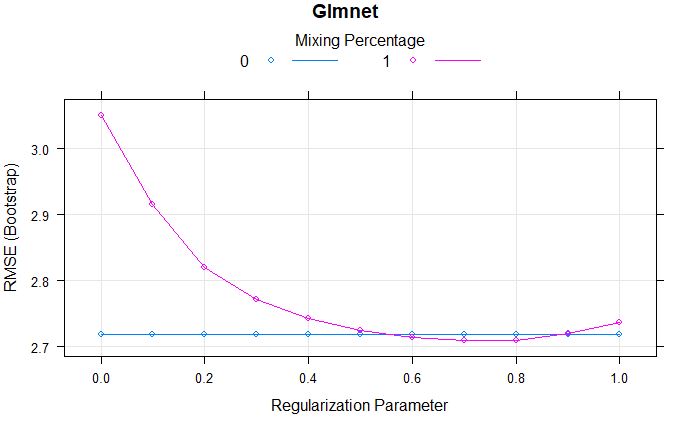
From the above comparison model, we can say that the lamda of 0.9 has lowest RMSE.
Full regularization path
plot(glmnetFit$finalModel)
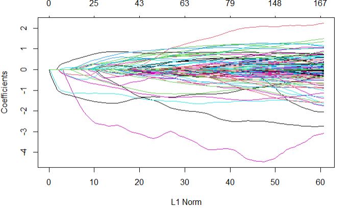
Next, we can plot the important predictors in this model based on their calculated importance scores using varImp function.
plot(varImp(glmnetFit), top = 20)
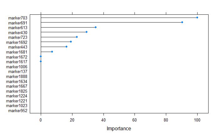
marker703 was calculated as the most important variable by glmnet model, which is consistent with random forest model. However, the glmnet has very few variables listed in comparison to rf.
Validation of glmnet model
Now we can test the robustness of the glmnet model by testing it on test_set data set, and regressing the predicted and measured values.
prediction_glmnet <- predict(glmnetFit, test_set)

plot(test_set$phenotype, prediction_glmnet,
     main = "GLMnet", pch=17, col=c("red"))
abline(lm(prediction_glmnet~test_set$phenotype))
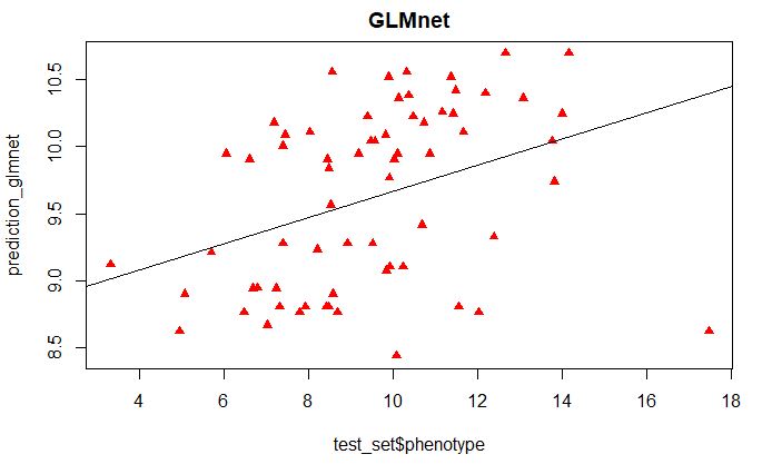
From the above plot, we see that the most important variables only classify the high and low phenotypic scores as categorical variables, which is not the nature of this phenotype data used in this tutorial.
And we can also calculate the RMSE between the predicted and measured values.
error_glm <- prediction_glmnet - test_set$phenotype
rmse_glm <- sqrt(mean(error_glm^2))
rmse_glm
Scatter plots of the predicted values from two models
plot(test_set$phenotype, prediction_glmnet,
      pch=17, col=c("red"), ylab = "Predicted", xlab = "Measured")
points(test_set$phenotype, prediction_rf, pch=20, col=("blue"))
abline(lm(prediction_glmnet~test_set$phenotype), lwd=1, col="red")
abline(lm(prediction_rf~test_set$phenotype), lwd=1, col="blue")
legend(14,9, legend=c("GLMnet", "Random Forest"),
       col=c("red", "blue"), lty=1, cex=0.8)
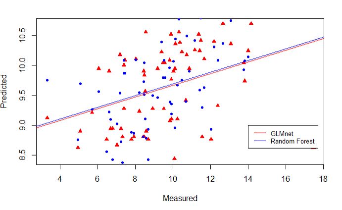
Comparing the Random Forest and Glmnet models
We can compare the performance of the models by studying their MAE, RMSE and R-squared values side-by-side, making it very convenient.
# Create model_list
model_list <- list(random_forest = randomForestFit, glmnet = glmnetFit)

# Pass model_list to resamples(): resamples
resamples <- resamples(model_list)
resamples

# Summarize the results
summary(resamples)
Output:
Call:
 summary.resamples(object = resamples)

 Models: random_forest, glmnet
 Number of resamples: 25

 MAE
                   Min.  1st Qu.   Median     Mean  3rd Qu.     Max. NA's
 random_forest 1.827043 1.955185 2.227830 2.159293 2.325698 2.462633    0
 glmnet        1.906341 2.115096 2.219258 2.256743 2.358562 2.839599    0

 RMSE
                   Min.  1st Qu.   Median     Mean  3rd Qu.     Max. NA's
 random_forest 2.251769 2.464010 2.697926 2.668136 2.850605 3.100536    0
 glmnet        2.323055 2.544948 2.697235 2.724706 2.819970 3.509943    0

 Rsquared
                       Min.    1st Qu.   Median      Mean   3rd Qu.      Max.
 random_forest 4.784201e-02 0.07672433 0.117394 0.1296488 0.1714565 0.3358213
 glmnet        8.322920e-07 0.06500280 0.126212 0.1350947 0.1709628 0.4315585
               NA's
 random_forest    0
 glmnet           0
From above table, we can tell that the random forest model appears to be better model incoparison to glmnet.
plot models by MAE, R-squrared and RMSE
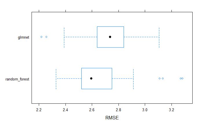
Similarly, we can visually inspect the models accuracies.
bwplot(resamples, metric = "RMSE")
dotplot(resamples, metric = "RMSE")
Conclusion:
In this tutorial, real genetic markers and phenotype data were used in machine learning models: random forest and glmnet(lasso and ridge regression). Marker data were converted into numeric format and numerically imputed, prior to performing the supervised machine learning. Both models had a very close performance for this data set, but random forest did perform slightly better in comparison to glmet, and most importantly both models listed marker703 as the most important variable, which is astoudingly consistent with my QTL analysis, that is the peak QTL marker was in LD with marker703 explaining highest phenotypic variance.