Building genetic maps can be challenging and sometimes quite stressful, especially, when dealing with thousands or even millions of markers. In this post, I am hoping to help anyone who would like to get started to build a decent genetic map in an open software Lep-MAP3 , and finally, evaluating the accuarcy of the genetic map and plotting it.
Table of contents
- QC analysis
- Install LepMap3
- Running LepMap modules
- Convert Phased data into Gnenotyes
- 4way-Cross rQTL
- Validate Genetic Map
- Plot in MapChart
Note: If you have an amplicon sequencing (AmpSeq or rhAmpSeq) haplotype data, you can convert the data into a psuedo VCF file using Haplotype to VCF PERL script.
Quality control analysis
Prior to building genetic maps - I strongly advise to perform QC analysis on your genetic data.
There are two QC tests that i usually perform: 1) Multidimensional scaling (MDS) and 2) Check for Mendelian Error
Click here for Multidimensional scaling (MDS) tutorial.
Click here for Mendelian Error Check tutorial.
How to transfer files using FileZilla
Please watch below video to: download , install and configure FileZilla. It will show you how to upload files and folders to your server.
Installing Lep-MAP3
The Lep-MAP3 software is built in Linux and one has to have some experience in working in command-line environment.
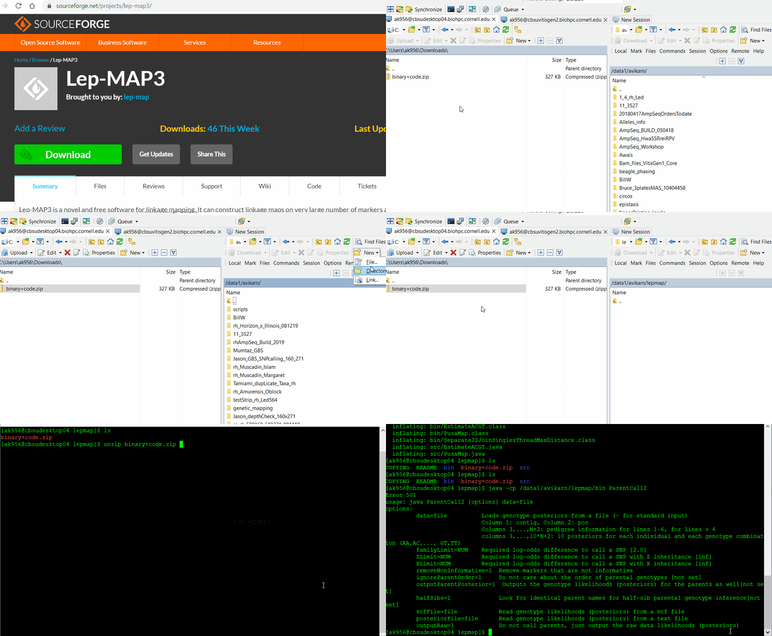
Downloand and install Lep-Map3 on your computer following below steps:
Running Lep-MAP3
The steps invloved in the genetic mapping process in Lep-MAP3 are shown in the flow chart below.

Step 1.1. File Preparation
Important - Correctly install the Lep-MAP3 software on your computer, and please make sure its the latest version. There are two files that are required as input files:
Download sample genotype file (VCF) here.
Download sample Pedigree file (.txt) here.

Step 1.2. Parent Call
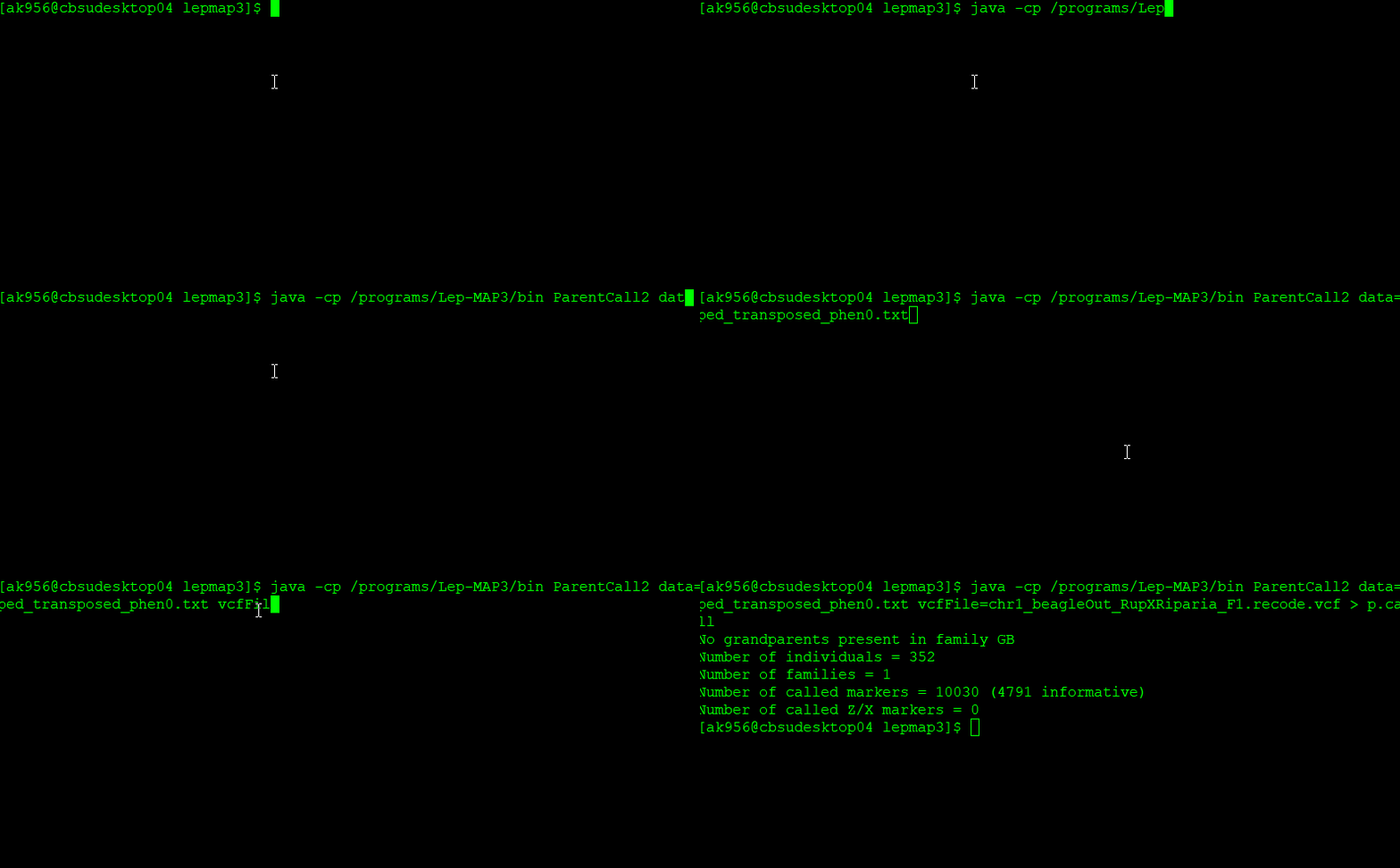
The parental genotypes are called using the ParentCall2 module, using the below command:
$ java -cp [path]/Lep-MAP3/bin ParentCall2 data = pedigree.txt vcfFile = File.vcf > p.call
Note: path is the directory where Lep-MAP3 is located on your computer.
Step 1.3. Filtering
This an optional step - However, One may use the Filtering2 module to remove non-informative markers (Markers that are monomorphic or homozygous in both parents), and distorted markers (markers segregating in a non-Mendelian fashion) using the below command line:
$ java -cp /path/Lep-MAP3/bin Filtering2 data=p.call removeNonInformative=1 dataTolerance=0.0000001 > p_fil.call
Note: Use the parameter removeNonInformative to remove markers that are homozygous/monomorphic, and dataTolerance to remove distorted markers at given p-value threshold.
Step 1.4. Separate Chromosomes
In this step, SeparateChromosomes2 module is used to categorize markers into linkage groups (LGs) using the below command:
$ java -cp /path/Lep-MAP3/bin SeparateChromosomes2 data=p_fil.call lodLimit=5 > map.txt
Note: One can use parameters such as lodLimit and theta to split the linkage groups.
One can check the number of markers in the in map file using the below command:
$ sort map.txt|uniq -c|sort -n
Step 1.5. Order Markers
In this step, markers separated into their corresponding linkage groups are ordered using OrderMarkers2 module using the below command:
$ java -cp /path/Lep-MAP3/bin OrderMarkers2 data=p_fil.call map=map.txt > order.txt
One may use the parameter sexAveraged to calculate sex-averaged map distances (by default male and female genetic maps are curated), also numMergeIterations parameter can be used to adjust number of iterations (by deafault its 6 iterations per linkage group).
2.0 Checking the accuracy of the marker order
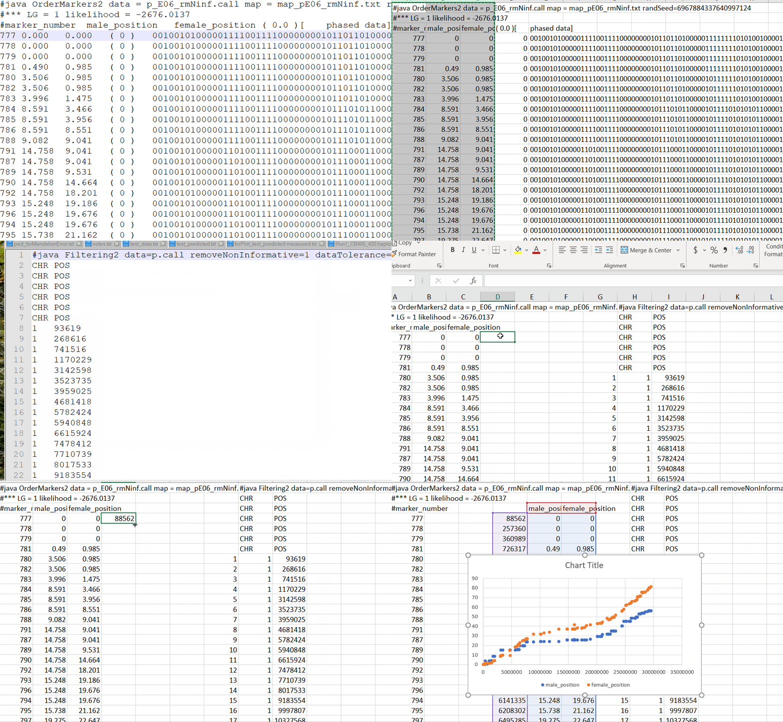
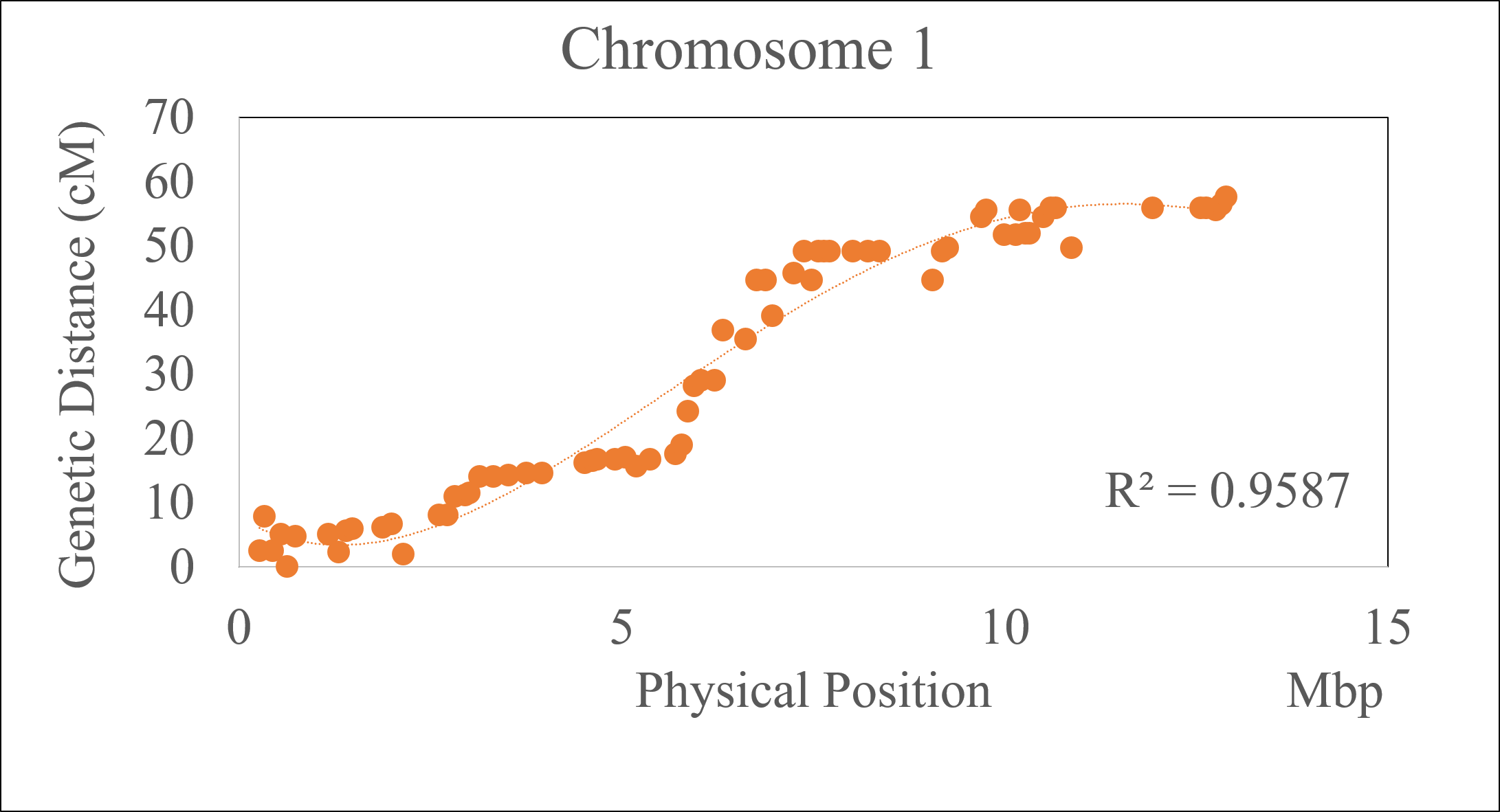
If the physical positons of the markers in the curated genetic map curation are known, then one may use that information to evaluate the quality of the marker order in the genetic map, especially markers that inflate the chromosome length, by making a correlation plot of the genetic and physical positions of the markers for each chromosome or linkage group.
Note: It is a common scenario to see the marker orders are flipped relative to their physical positions. There is nothing to panic about, one may fix it by manually sorting it.
Command to obtain the marker information using cut:
cut -f1,2 p.call > cut_pcall.txt
Note: Please make sure to use the p.call file that you used in the ordering step!
Follow the below steps to perform the correlation analysis:
3.0 Converting phased output data from OrderMarkers2 to genotypes
The phased data from OrderMarkers2 step can be converted to fully informative “genotype” data by using map2gentypes.awk script and command below:
Download the map2gentypes.awk script here.
Next, run the map2genotypes.awk script by following the command shown below.
$ awk -vfullData=1 -f map2genotypes.awk order.txt > genotypes.txt
Snippet of the map2gentypes.awk output:
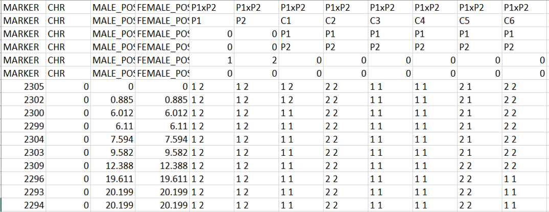
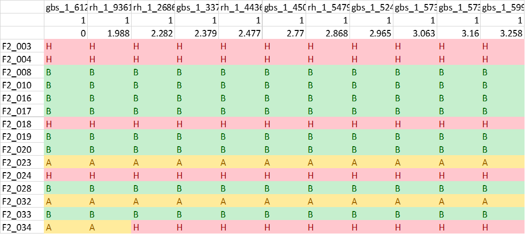
One may convert the genotypes in 1 1 => A, 2 2 => B, 1 2 or 2 1 => H format (See below figure) in MS Excel using Find and Replace function, which can be then be loaded in R/Qtl for QTL mapping.
LepMap3 imputes and phase the genotype calls, therefore, A and B allele represent major and minor allele frequencies and it will change from parent/phase. They do not represent one specific parent and information depends on the parent and the phase of the marker.
Covnvert genotype data into 4-way cross RQtl input data
In case both parents are heterozygotes, the cross is a 4way cross, also know as AB x CD phased output data from OrderMarkers2 (1 1, 12, 21, 22) into Rqtl 4way code that 1, 2, 3 and 4 as shown in the below table. Also, please remember, in LepMap pedigree file: male parent = 1 , female parent = 2, and first digit of the phased genotypes is inherited from paternal parent and the second from maternal parent.
Read more on genotype file formatting here: https://github.com/kbroman/qtl/blob/main/man/read.cross.Rd
LepMap	RQtl-4way-code	RQtl genotype
1 1	1	AC
1 2	2	BC
2 1	3	AD
2 2	4	BD
Finally import the converted the 4-waycross genetic map in RQTL using the below command:
 GenoData = read.cross(format = "csv", file = "geneticMap.csv", genotypes=NULL,
                     estimate.map = F, crosstype="4way")
4.0 Validate the genetic map by conducting QTL analysis
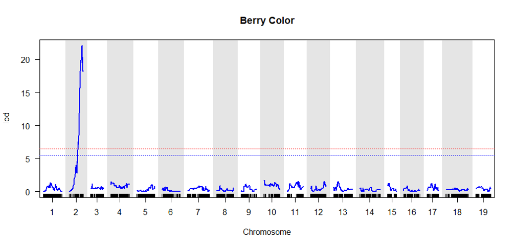
It is a good QC step to perform a QTL analysis of a well studied trait to check if expected QTL region is observed in the curated genetic mmap
Click here for QTL mapping tutorial.
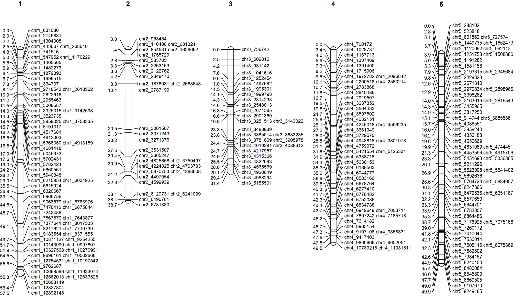
5.0 Graphical presentation of linkage maps in Mapchart
Software Mapchart can be downloaded from below link. https://www.wur.nl/en/show/Mapchart.htm
Click here for Mapchart tutorial.
Thank you for reading this tutorial. I really hope these steps will get you started in genetic map construction in Lep-MAP3. The key is to PRACTISE. . If you have any comments or suggestions, please let comment below or send me an email.
Happy mapping !
Bibliography
Rastas, Pasi. “Lep-MAP3: robust linkage mapping even for low-coverage whole genome sequencing data.” Bioinformatics 33.23 (2017): 3726-3732.